Download
1 / 95
960 likes | 1.06k Views
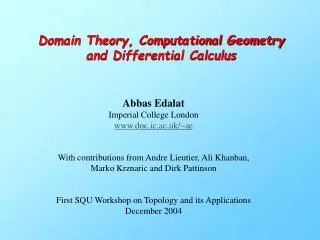
Domain Theoretic Models of Geometry and Differential Calculus. Abbas Edalat Imperial College http://www.doc.ic.ac.uk/~ae. Joint work with Andre Lieutier Dassault Systemes. With contributions from Ali Khanban, Marko Krznaric. ISDT 2001 Chengdu, China.

E N D
Domain Theoretic Models of Geometry and Differential Calculus Abbas Edalat Imperial College http://www.doc.ic.ac.uk/~ae Joint work with Andre Lieutier Dassault Systemes With contributions from Ali Khanban, Marko Krznaric ISDT 2001 Chengdu, China
Computational Model for Classical Spaces x {x} X Classical Space DXDomain • A research project since 1993: Reconstruct basic mathematics! • Embed classical spaces into the set of maximal elements of suitable domains
Computational Model for Classical Spaces Previous Applications: • Fractal Geometry New algorithms for computing fractal objects • Measure & Integration Theory The Generalized Riemann Integral • Exact Real Arithmetic C-library based on linear fractional transformations for Computation of Elementary Functions
Part 1: A Domain-Theoretic Model of Geometry To develop a Computable model for Geometry and Solid Modelling, so that: the model is mathematically sound, realistic; the basic building blocks are computable; it bridges theory and practice.
Why do we need a data type for solids? Answer: To develop robust algorithms! Lack of a proper data type and use of real RAM in which comparison of real numbers is decidable give unreliable programs in practice!
The Intersection of two lines With floating point arithmetic, find the point P of the intersection L1L2. Then:min_dist(P, L1) > 0,min_dist(P, L2) > 0.
The Convex Hull Algorithm A, B & Cnearly collinear With floating point we can get:
The Convex Hull Algorithm A, B & Cnearly collinear With floating point we can get: (i)AC, or
The Convex Hull Algorithm A, B & Cnearly collinear With floating point we can get: (i)AC, or (ii) justAB, or
The Convex Hull Algorithm A, B & Cnearly collinear With floating point we can get: (i)AC, or (ii) justAB,or (iii) justBC, or
The Convex Hull Algorithm A, B & Cnearly collinear With floating point we can get: (i)AC, or (ii) justAB, or (iii) justBC, or (iv) none of them. The quest for robust algorithms is the most fundamental unresolved problem in solid modelling and computational geometry.
A Fundamental Problem in Topology and Geometry • Subset A X topological space.Membership predicate A : X {tt, ff } is continuous iff A is both open and closed. In particular, for A Rn, A , A RnA : Rn {tt, ff } is not continuous. Most engineering is done, however, in Rn.
Non-computability of the Membership Predicate This predicate is not computable: If x is on the boundary, we cannot in general determine if it is in or out at any finite stage of computation. There is discontinuity at the boundary of the set. True False
Non-computable Operations in Classical CG & SM • A: Rn{tt, ff} not continuous means it is not computable, even for simple objects like A=[0,1]n. • x Ais not decidable even for simple objects: for A = [0,) R, we just have the undecidability of x 0. • The Boolean operation is not continuous, hence noncomputable, wrt the natural notion of topology on subsets: : C(Rn) C(Rn) C(Rn),whereC(Rn)iscompact subsets with the Hausdorff metric.
This is Really Ironical! • Topology and geometry have been developed to study continuous functions and transformations on spaces. • The membership predicate and the binary operation for are the fundamental building blocks of topology and geometry. • Yet, these fundamental functions are not continuous in classical topology and geometry.
Elements of a Computable Topology/Geometry open open • Redefine: A : X {tt, ff} with the Scott topology on {tt, ff}. tt ff observable observable Non-observable • The membership predicate A : X {tt, ff} fails to be continuous on A, the boundary of A. • For any open or closed set A, the predicate x A is non-observable, like x = 0. A is now a continuous function.
Elements of a Computable Topology/Geometry • Note that A=B iff int A=int B & int Ac=int Bc, i.e. sets with the same interior and exterior have the same membership predicate. • We now change our view: In analogy with classical set theory where every set is completely determined by its membership predicate, we define a (partial) solid object to be given by any continuous map: f : X { tt, ff } • Then:f –1{tt} is open; it’s called the interior of the object. f –1{ff} is open; it’s called the exterior of the object.
Partial Solid Objects • We have now introduced partial solid objects, since X \ (f –1{tt} f –1{ff}) may have non-empty interior. • We partially order the continuous functions:f, g : X {tt, ff } f⊑g x X . f(x) ⊑ g(x) • f ⊑g f –1{tt} g –1{tt} & f –1{ff} g –1{ff}Therefore, f⊑g means g has more information about an idealized real solid object.
The Geometric (Solid) Domain of X • The geometric (solid) domainS (X) of X is the poset (X {tt, ff }, ⊑ ) • S(X) is isomorphic to the poset SO(X) of pairs of disjoint open sets (O1,O2) ordered componentwise by inclusion:
Properties of the Geometric (Solid) Domain • Theorem If X is Hausdorff, then: (O1, O2) Maximal (SX, ⊑) iff O1= int O2c & O2= int O1c. This is a regular solid object: O1=int O1 & O2=int O2 • Definition (O1, O2) , O1 ≠∅≠O2 ,is a classical object if O1 ∪ O2 = X. • TheoremFor a second countable locally compact Hausdorff space X(e.g. Rn), S(X) is bounded complete and –continuous with (U1, U2) << (V1, V2) iff the closures ofU1 and U2 are compact subsets ofV1andV2 respectively.
Examples • B = {xR2 ⃒ |x| ≤ 1}represented by({x⃒ |x| < 1} , {x⃒ |x| > 1}) Maximal (SR2, ⊑)is a regular solid object. • A = {xR2 ⃒ |x| ≤ 1} [1, 2]represented in the model by(int A, int Ac) = ( {x⃒ |x| < 1}, R2\A )is a classical (but non-regular) solid object.
Boolean operations and predicates Theorem All these operations are Scott continuous and preserve classical solid objects.
Subset Inclusion Let Subset inclusion is Scott continuous.
General Minkowski operator • For smoothing out sharp corners of objects. • SbRn = { (A, B) SRn | Bc is bounded} ∪{(∅,∅)}. All real solids are represented in SbRn. • Define:__ : SRnSbRn SRn ((A,B) , (C,D)) ↦ (A ⊕ C , (Bc ⊕ Dc)c) where A ⊕ C = { a+c | a A, c C } • Theorem __ is Scott continuous.
An effectively given solid domain • The geometric domain SX can be given effective structure for any locally compact second countable Hausdorff space, e.g. Rn, Sn, Tn, [0,1]n. • Consider X=Rn. The set of pairs of disjoint open rational polyhedra of the form K = (L1 , L2) , with L1 L2 = , gives a basis for SX. • Let Kn= (π1(K n ) , π2(K n) ) be an enumeration of this basis. • (A, B) is a computable partial solid objectif there exists a total recursive function ß:NN such that: (A , B) = ( ∪n π1(Kß(n) ) , ∪n π2(Kß(n) ) )
Computing a Solid Object • In this model, a solid object is represented by its interior and exterior. • The interior and the exterior are approximated by two nested sequence of rational polyhedra.
Computable Operations on the Solid Domain • F: (SX)n SX or F: (SX)n { tt, ff } is computable if it takes computable sequences of partial solid objects to computable sequences. • Theorem All the basic Boolean operations and predicates are computable wrt any effective enumeration of either the partial rational polyhedra or the partial dyadic voxel sets.
Quantative Measure of Convergence • In our present model for computable solids, there is no quantitative measure for the convergence of the basis elements to a computable solid. • Example: The minimum distance from say a rational point to a computable solid is semi-computable, but not computable. • We will enrich the notion of domain-theoretic computability to include a quantitative measure of convergence.
Hausdorff Computability • (A , B) S [–k, k]n is Hausdorff computable if there exists an effective chain Kß(n) of basis elements with ß :NN a total recursive function such that: (A , B) = ( ∪n π1(Kß(n) ) , ∪n π2(Kß(n) ) ) with d (π1(Kß(n) ) ,A ) < 1/2n , d (π2(Kß(n) ) ,B) < 1/2n • We strengthen the notion of a computable solid by using the Hausdorff distance d between compact sets in Rn. • d(C,D) = min{ r | C Dr & D Cr } where Dr = { x | y D. |x-y| r }
Hausdorff computability • Two solid objects which have a small Hausdorff distance from each other are visually close. • The Hausdorff distance gives a natural quantitative measure for approximation of solid objects. • However, the intersection or union of two Hausdorff computable solid objects may fail to be Hausdorff computable. • Examples of such failure are nontrivial to construct.
Boolean Intersection is not Hausdorff computable is Hausdorff computable. However: Q([0,1] {0})= [r,1] {0} R2is not Hausdorffcomputable.
Lebesgue Computability • (A , B) S [–k, k]d is Lebesgue computable iff there exists an effective chain Kß(n) of basis elements with ß :NNa total recursive functions such that: (A , B) = ( ∪n π1(Kß(n) ) , ∪n π2(Kß(n) ) ) µ(A) - µ(π1(Kß(n) ) ) < 1/2n & µ(B) - µ(π2(Kß(n) ) ) < 1/2n • A function isLebesgue computableif it preserves Lebesgue computable sequences. • Theorem Boolean operations are Lebesgue computable.
Hausdorff and Lebesgue computability 0 1 s0 • Hausdorff computable ⇏Lebesgue computableComplement of a Cantor set with Lebesgue measure 1– r withr =lim rn: left computable but non-computable real. start with stage 1 stage 2 • At stage n remove 2n open mid-intervals of length sn/2n.
Hausdorff and Lebesgue computability Then [r,1] {0} R2 is Lebesgue computable but not Hausdorff computable. • Lebesgue computable ⇏ Hausdorff computable Let 0 <rn Qwithrn↗ r, left computable, non-computable 0 < r < 1.
Hausdorff and Lebesgue Computable Objects • Hausdorff computable ⇏Lebesgue computable • Lebesgue computable ⇏ Hausdorff computable • Theorem: A regular solid object is computable iff it is Hausdorff computable. • However: A computable regular solid object may not be Lebesgue computable.
Conclusion Our model satisfies: • A well-defined notion of computability • Reflects the observable properties of geometric objects • Is closed under basic operations • Captures regular and non-regular sets • Supports a methodology for designing robust algorithms
Part 2: Data-types for Computational Geometry and Systems of Linear Equations The Convex Hull Voronoi Diagram or the Post Office problem The Partial Circle through three partial points Partial Lines and Projective Geometry: the intersection of hyper-planes, the solution of systems of linear equations
The Inner Convex Hull Algorithm Top left corners Top right corners bottom left corners bottom right corners
The Convex Hull map T3 T2 Each rectangle TIR2 has vertices T1,T2,T3,T4, going anti-clockwise from the right bottom corner. T4 T1 • Let Hm: (R2)m C(R2) be the classical convex Hull map, with C(R2) the set of compact subsets of R2, with the Hausdorff metric. • Let(IR2, ) be the domain of rectangles in R2. • For x=(T1,T2,…,Tm)(IR2)m, define: Cm : (IR2)m SR2,Cm(x)=(Im(x),Em(x)) with: Em(x):={Hm(y) | y(R2)m, yiTi, 1 I m} Im(x):={Hm(y) | y(R2)m, yiTi, 1 I m}
The Convex Hull is Computable! • Proposition: Em(x)=(H4m((Ti1,Ti2,Ti3,Ti4))1im)c Im(x)=Int({Hm((Tin))1im) | n=1,2,3,4}). • Theorem: The map Cm : (IR2)m SR2is Scott continuous, Hausdorff and Lebesgue computable. • Complexity: • Em(x) is O(m log m). • Im(x) is also O(m log m). We have precisely the complexity of the classical convex hull algorithm in R2 and R3.
Voronoi Diagrams We are given a finite number of points in the plane. Divide the plane into components closest to these points. • This problem is equivalent to the Delaunay triangulation of the points: (1) Triangulate the set of given points so that the interior of the circumference circles do not contain any of the given points. (2) Draw the perpendicular bisectors of the edges of the triangles.
Voronoi Diagram & Partial Circles • Recall that the Voronoi diagram is dual to the Delaunay triangulation: Given a finite number of points of the plane find the triples of points so that the interior of the circle through any triple does not contain any other points. . . . . . . • The centre of the circle through the three vertices of a triangle is the intersection of the perpendicular bisectors of the three edges of the triangle. The partial circle of three partial points in the plane is obtained by considering the Partial Perpendicular Bisectorof two partial points in the plane.
PPBs for Three Partial Points Partial Centre