Download
1 / 19
190 likes | 295 Views
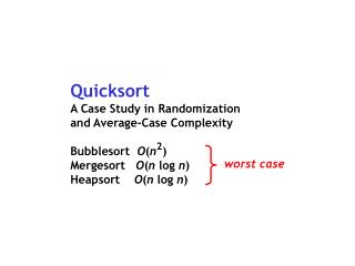
Probability theory and average-case complexity. Review of probability theory. Review of probability theory: outcome. Examples: Rolling a die and getting 1 Rolling a die and getting 6 Flipping three coins and getting H, H, T Drawing two cards and getting 7 of hearts, 9 of clubs

E N D
Review of probability theory:outcome • Examples: • Rolling a die and getting 1 • Rolling a die and getting 6 • Flipping three coins and getting H, H, T • Drawing two cards and getting 7 of hearts, 9 of clubs • NOT examples: • Rolling a 6-sided die and getting an even number (this is more than one outcome—3 to be exact!) • Drawing a card and getting an ace (4 outcomes!)
Review of probability theory:event • Defn: one or more possible outcomes • Examples: • Rolling a die and getting 1 • Rolling a die and getting an even number • Flipping three coins and getting at least 2 “heads” • Drawing five cards and getting one of each suit
Review of probability theory:sample space • Defn: A set of events • Examples: Drawing a card Flipping 3 coins Rolling 2 dice
Review of probability theory:probability distribution • Idea: take a sample space S and add probabilities for each event • Defn: mapping from events of S to real numbers • for any event A in S • = 1 • Example: 0.753 0.75*0.75 0.75 0.752*0.25 0.752*0.25 0.75*0.25 0.75*0.252 Flipping 3 biased coins75% heads, 25% tails 0.25*0.75 0.752*0.25 0.25 0.75*0.252 0.75*0.252 0.253 0.25*0.25
Review of probability theory:probability of an event A • Defn: • Example: • Pr(roll a die and get even number) = Pr(roll a 2) + Pr(roll a 4) + Pr(roll a 6)
Review of probability theory:random variable • Idea: turn events into numbers • Let S be a sample space • Defn: mapping from events to real numbers • Example: X = the number on a die after a rollevent “rolling a 1” -> 1event “rolling a 2” -> 2…event “rolling a 6” -> 6 Technically, X is a function,so we can write:X(rolling a 1) = 1 X(rolling a 2) = 2…X(rolling a 6) = 6
Review of probability theory:expected value of a random variable • Idea: “average” value of the random variable • Remember: random variable X is a mapping from events in a sample space S to numbers • Defn: Expected value of • Short form: • Example: X = number on die after rolling Here, x = X(event)
Expected running time of an algorithm • Let A be an algorithm. • Let Sn be the sample space of all inputs of size n. • To talk about expected (/average) running time, we must specify how we measure running time. • We want to turn each input into a number (runtime). • Random variables do that… • We must also specify how likely each input is. • We do this by specifying a probability distribution over Sn.
Expected running time of an algorithm • Recall: algorithm A, sample space Sn • We define a random variabletn(I)= number of steps taken by A on input I • We then obtain: • In this equation, I is an input in Sn, andPr(I) is the probability of input I according to the probability distribution we defined over Sn • is the average running time of A, given Sn
Example time: searching an array • Let L be an array containing 8 distinct keys Search(k, L[1..8]): for i = 1..8 if L[i].key == k then return true return false • What should our sample space S9 of inputs be? • Hard to reason about all possible inputs. • (In fact, there are uncountably infinitely many!) • Can group inputs by how many steps they take!
Grouping inputs by how long they take Search(k, L[1..8]): for i = 1..8 if L[i].key == k then return true return false • What causes us to return in loop iteration 1? • How about iteration 2? 3? … 8? After loop? • S9 = {“k is in L[1]”, “k is in L[2]”, …, “k is in L[8]”, “k is not in L”} • Now we need a random variable for S9!
Using a random variableto capture running time Search(k, L[1..8]): for i = 1..8 if L[i].key == k then return true return false • S9 = {“k is in L[1]”, “k is in L[2]”, …, “k is in L[8]”, “k is not in L”} • Let T(I) = running time for input I in S9 • T(“k is in L[1]”) = 2, T(“k is in L[2]”) = 4, …, T(“k is in L[i]”) = 2i, T(“k is not in L”) = 2*8+1 = 17 • We then obtain: Do we have enough information to compute an answer? For simplicity: assume each iteration takes 2 steps. 1 step
What about a probability distribution? • We have a sample space and a random variable. • Now, we need a probability distribution. • This is given to us in the problem statement. • For each i, • If you don’t get a probability distribution from the problem statement, you have to figure out how likely each input is, and come up with your own.
Computing the average running time • We now know: • T(I) = running time for input I in S9 • T(“k is in L[i]”) = 2i T(“k is not in L”) = 17 • S9 = {“k is in L[1]”, “k is in L[2]”, …, “k is in L[8]”, “k is not in L”} • Probability distribution: • For each i, • Therefore:
The final answer • Recall: T(“k is in L[i]”) = 2i, T(“k is not in L”) = 17 • For each i, • Thus, the average running time is 13.