Download
1 / 7
70 likes | 130 Views
Stage 2 Presentation MAS2317 Katie Allman.

E N D
Stage 2 Presentation MAS2317 Katie Allman
A “degassing burst” is a seismic event that can occur just before a major earthquake. Let θ be the chance that a major earthquake will occur after a degassing burst has taken place. From discussions with a seismologist, we are able to elict the following: Pr(θ<0.6)=10-3 The seismologist also tells us that she thinks the most likely value for θ will be about 0.9. Use this information to justify using a Beta(22.6, 3.4) prior for θ, clearly explaining your method.
Prior Elicitation – the process by which we attempt to construct the most suitable prior distribution for θ. Substantial Prior Knowledge – turning expert opinion into a probability distribution for θ. I know to use a Beta Be(a, b) distribution (a > 0, b > 0) for θ, because the parameter of interest is a probability. E(θ) = Var(θ) = Mode(θ) =
We were told that the mode of the distribution should be around 0.9, therefore using the previous equation we have:
We were also told that Pr(θ<0.6)=10-3 which means when I integrate the pdf for the beta function between 0 and 0.6, I would get 0.001. i.e. By plugging in the value of a into this equation, I was then able to solve for b using R.
Using the command pbeta(x,a,b) and rearranging the previous equation (i.e. so it equals to 0), I obtained the following function: where here x = 0.6 is the value at which the cumulative distribution function is evaluated. I then used a numerical procedure to find the root of ‘answer’ in the R function. That is: I chose the specified domain as 1 to 100 because a,b>1.
Thus, the solution to the equation is , and by substituting this into I obtained Therefore a Beta(22.6, 3.4) distribution would be the best prior for θ.