John Dudley Université de Franche-Comté, Institut FEMTO-ST CNRS UMR 6174, Besançon, France

1. Supercontinuum to solitons: extreme nonlinear structures in optics John Dudley Université de Franche-Comté, Institut FEMTO-ST CNRS UMR 6174, Besançon, France

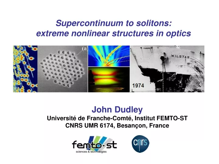
2. Supercontinuum to solitons: extreme nonlinear structures in optics Goery Genty Tampere University of Technology Tampere, Finland Fréderic Dias ENS Cachan France UCD Dublin, Ireland Bertrand Kibler, Christophe Finot,Guy Millot Université de Bourgogne, France Nail Akhmediev Research School of Physics & Engineering, ANU , Australia

3. Context and introduction • The analysis of nonlinear guided wave propagation in optics reveals features more commonly associated with oceanographic “extreme events” • Challenges – understand the dynamics of the specific events in optics – explore different classes of nonlinear localized wave – can studies in optics really provide insight into ocean waves? • Emergence of strongly localized nonlinear structures • Long tailed probability distributions i.e. rare events with large impact

4. Extreme ocean waves • Rogue Waves are large (~ 30 m) oceanic surface waves that represent statistically-rare wave height outliers • Anecdotal evidence finally confirmed through measurements in the 1990s 1934 1974 1945 Drauper 1995

5. Extreme ocean waves • There is no one unique mechanism for ocean rogue wave formation • But an important link with optics is through the (focusing) nonlinear Schrodinger equation that describes nonlinear localization and noiseamplification through modulation instability Cubic nonlinearity associated with an intensity-dependent wave speed - nonlinear dispersion relation for deep water waves - consequence of nonlinear refractive index of glass in fibers NLSE

6. (Extreme ocean waves) Ocean waves can be one-dimensional overlong and short distances … We also see importanceof understanding wavecrossing effects We are considering how muchcan in principle be containedin a 1D NLSE model

7. Rogue waves as solitons - supercontinuum generation

8. Rogue waves as solitons - supercontinuum generation

9. Supercontinuum physics • Modeling the supercontinuum requires NLSE with additional terms Essential physics = NLSE + perturbations Linear dispersion Self-steepening SPM, FWM, Raman Three main processes Soliton ejection Raman – shift to long l Radiation – shift to short l

10. Supercontinuum physics • Modeling the supercontinuum requires NLSE with additional terms Essential physics = NLSE + perturbations Linear dispersion Self-steepening SPM, FWM, Raman Three main processes Soliton ejection Raman – shift to long l Radiation – shift to short l

11. Spectral instabilities • With long (> 200 fs) pulses or noise, the supercontinuum exhibits dramatic shot-to-shot fluctuations underneath an apparently smooth spectrum Stochastic simulations 5 individual realisations (different noise seeds) Successive pulses from a laser pulse train generate significantly different spectra Laser repetition rates are MHz - GHz We measure an artificially smooth spectrum 835 nm,150 fs 10 kW, 10 cm

12. Spectral instabilities • Initial “optical rogue wave” paper detected these spectral fluctuations Schematic Stochastic simulations Time Series Histograms

13. Dynamics of “rogue” and “median” events is different • Differences between “median” and “rogue” evolution dynamics are clear when one examines the propagation characteristics numerically

14. Dynamics of “rogue” and “median” events is different • Differences between “median” and “rogue” evolution dynamics are clear when one examines the propagation characteristics numerically • But the rogue events are only “rogue” in amplitude because of the filter • Deep water propagating solitons unlikely in the ocean Dudley, Genty, Eggleton Opt. Express 16, 3644 (2008) ; Lafargue, Dudley et al. Electronics Lett. 45 217 (2009) Erkinatalo, Genty, Dudley Eur. Phys J. ST 185 135 (2010)

15. More insight from the time-frequency domain • gate • pulse • Ultrafast processes are conveniently visualized in the time-frequency domain • We intuitively see the dynamicvariation in frequency with time Spectrogram / short-time Fourier Transform pulsevariable delay gate Foing, Likforman, Joffre, Migus IEEE J Quant. Electron 28 , 2285 (1992) ; Linden, Giessen, Kuhl Phys Stat. Sol. B 206, 119 (1998)

16. More insight from the time-frequency domain • gate • pulse • Ultrafast processes are conveniently visualized in the time-frequency domain Spectrogram / short-time Fourier Transform pulsevariable delay gate Foing, Likforman, Joffre, Migus IEEE J Quant. Electron 28 , 2285 (1992) ; Linden, Giessen, Kuhl Phys Stat. Sol. B 206, 119 (1998)

17. Median event – spectrogram • “Median” Event

18. Rogue event – spectrogram

19. What can we conclude? • The extreme frequency shifting of solitons unlikely to have oceanic equivalent • BUT ... dynamics of localization and collision is common to any NLSE system MI

20. Early stage localization • The initial stage of breakup arises from modulation instability (MI) • A periodic perturbation on a plane wave is amplified with nonlinear transfer of energy from the background • MI was later linked to exact dynamical breather solutions to the NLSE Akhmediev & Korneev Theor. Math. Phys. 69, 1089-1093 (1986) Whitham, Bespalov-Talanov, Lighthill, Benjamin-Feir (1965-1969) Akhmediev-Korneev Theor. Math. Phys 69 189 (1986)

21. Early stage localization • Simulating supercontinuum generation from noise sees pulse breakup through MI and formation of Akhmediev breather (AB) pulses • Experimental evidence can be seen in the shape of the spectrum : simulation ------ : AB theory Temporal Evolution and Profile

22. Experiments • Spontaneous MI is the initial phase of CW supercontinuum generation • 1 ns pulses at 1064 nm with large anomalous GVDallow the study of quasi-CW MI dynamics • Power-dependence of spectral structure illustratesthree main dynamical regimes Spontaneous MI sidebands Intermediate (breather) regime Supercontinuum Dudley et al Opt. Exp. 17, 21497-21508 (2009)

23. Comparing supercontinuum and analytic breather spectrum • Breather spectrum explains the “log triangular” wings seen in noise-induced MI

24. The Peregrine Soliton • Particular limit of the Akhmediev Breather in the limit of a 1/2 • The breather breathes once, growing over a single growth-return cycle and having maximum contrast between peak and background • Emergence “from nowhere” of a steep wave spike • Polynomial form 1938-2007

25. Under induced conditions we excite the Peregrine soliton • Two closely spaced lasers generate a low amplitude beat signal that evolves following the expected analytic evolution • By adjusting the modulation frequency we can approach the Peregrine soliton

26. Temporal localisation • Experiments can reach a = 0.45, and the key aspects of the Peregrine soliton are observed – non zero background and phase jump in the wings Nature Physics 6 , 790–795 (2010) ; Optics Letters 36, 112-114 (2011)

27. Spectral dynamics Signal to noise ratio allows measurements of a large number of modes

28. Early-stage collisions • Collisions in the MI-phase can also lead to localized field enhancement • Such collisions lead to extended tails in the probability distributions • Controlled collision experiments suggest experimental observation may be possible through enhanced dispersive wave radiation generation 3 breathercollisions 2 breather collisions Single breather Distance Time

29. Other systems Statistics of filamentation Lushnikov et al. OL (2010) Capillary rogue waves Shats et al. PRL (2010) Optical turbulence in a nonlinear optical cavity Montina et al. PRL (2009) Matter rogue waves Bludov et al. PRA (2010) Resonant freak microwaves De Aguiar et al. PLA (2011) Financial Rogue WavesYan Comm. Theor. Phys. (2010)

30. Conclusions and Challenges • Analysis of nonlinear guided wave propagation in optics reveals features more commonly associated with oceanographic “extreme events” • Solitons on the long wavelength edge of a supercontinuum have been termed “optical rogue waves” but are unlikely to have an oceanographic counterpart • The soliton propagation dynamics nonetheless reveal the importance of collisions, but can we identify the champion soliton in advance? • Studying the emergence of solitons from initial MI has led to a re-appreciation of earlier studies of analytic breathers • Spontaneous spectra, Peregrine soliton, sideband evolution etc • Many links with other systems governed by NLSE dynamics • Challenges – understand the dynamics of the specific events in optics – explore different classes of nonlinear localized wave – can studies in optics really provide insight into ocean waves?

31. Tsunami vs Rogue Wave Tsunami Rogue Wave

32. Tsunami vs Rogue Wave Tsunami Rogue Wave

33. Real interdisciplinary interest

34. Longitudinal localisation • Without cutting the fiber we can study the longitudinal localisation by changing effective nonlinear length • Characterized in terms of the autocorrelation function

35. More on localisation • Localisation properties can be readily examined in experiments as a function of frequency a • Define localisation measures in terms of temporal width to period and longitudinal width to period • Temporal • Longitudinal • determined numerically

36. Under induced conditions we enter Peregrine soliton regime • Localisation properties as a function of frequency a can be readily examined in experiments • Define localisation measures in terms of temporal width to period and longitudinal width to period • Temporal Spatial Spatio-temporal

37. Under induced conditions we enter Peregrine soliton regime • Localisation properties as a function of frequency a can be readily examined in experiments • Define localisation measures in terms of temporal width to period and longitudinal width to period • Temporal Spatial Spatio-temporal • Red region corresponds to previous experiments – weak localisationBlue region – our experiments – the Peregrine regime