Download
1 / 30
300 likes | 319 Views
DISTRIBUTED AND PARALLEL COMPUTING SKR 3202. Chapter 4 : Performance and Scalability of Parallel System (w6). TOPIC LEARNING OUTCOMES. Performance Evaluation Effect of Granularity and Data Mapping on Performance.

E N D
DISTRIBUTED AND PARALLEL COMPUTINGSKR 3202 Chapter 4 : Performance and Scalability of Parallel System (w6)
TOPIC LEARNING OUTCOMES • Performance Evaluation • Effect of Granularity and Data Mapping on Performance • Explain and analysis the performance metrics of parallel system(C1, A2) • Describe the basic concept of granularity and how it effects the parallel system(C4, P3) SKR 3202 :: Chapter 4
4.1 Performance Evaluation for Parallel System • It is important to study the performance of parallel programs with a view to determining the best algorithm, evaluating hardware platforms, and examining the benefits from parallelism. • A number of metrics have been used based on the desired outcome of performance analysis. • A sequential algorithm is evaluated by its runtime (in general, asymptotic runtime as a function of input size); the performance of algorithms applied to very large input datasets. • The parallel runtime of a program depends on the input size, the number of processors, and the communication parameters of the machine. Asymptotically i.e., as the input size goes to infinity. SKR 3202 :: Chapter 4
4.1 Performance Evaluation (cont.) • A number of performance measures are intuitive. • Wall clock time - the time from the start of the first processor to the stopping time of the last processor in a parallel ensemble. • But how does this scale when the number of processors is changed of the program is ported to another machine altogether? • How much faster is the parallel version? “If I use two processors, shouldn't my program run twice as fast?” • No - a number of overheads, including wasted computation, communication, idling, and contention cause degradation in performance. SKR 3202 :: Chapter 4 4
4.1 Performance Evaluation (cont.) • Serial runtime of a program • Refers to the time elapsed between the beginning and the end of its execution on a sequential computer. • The parallel runtime • Refers to the time that elapses from the moment the first processor starts to the moment the last processor finishes execution. • We denote the serial runtime by Ts and the parallel runtime by TP . SKR 3202 :: Chapter 4 5
4.1 Performance Evaluation : Parallel Overhead Let Tall be the total time collectively spent by all the processing elements. TS is the serial time. Observe that Tall - TS is then the total time spend by all processors combined in non-useful work. This is called the total overhead. The total time collectively spent by all the processing elements Tall = p TP (p is the number of processors). The overhead function (To) is therefore given by To = p TP - TS (1) SKR 3202 :: Chapter 4 6
4.1 Performance Evaluation : Speedup Speedup (S) is the ratio of the time taken to solve a problem on a single processor to the time required to solve the same problem on a parallel computer with p identical processing elements. Speedup can be as low as 0 (the parallel program never terminates). Speedup, in theory, should be upper bounded by p - after all, we can only expect a p-fold speedup if we use times as many resources. A speedup greater than p is possible only if each processing element spends less than time TS / p solving the problem. SKR 3202 :: Chapter 4 7
4.1 Performance Evaluation : Speedup (cont.) • Speedup can be referred as how much a parallel algorithm is faster than a corresponding sequential algorithm • Speedup is defined by the following formula: where: p is the number of processors T1 is the execution time of the sequential algorithm Tp is the execution time of the parallel algorithm with p processors SKR 3202 :: Chapter 4 8
4.1 Performance Evaluation : Speedup (cont.) • Example : • Consider the problem of parallel bubble sort. • The serial time for bubblesort is 150 seconds. • The parallel time for odd-even sort (efficient parallelization of bubble sort) is 40 seconds. • The speedup would appear to be 150/40 = 3.75. • But is this really a fair assessment of the system? • What if serial quicksort only took 30 seconds? In this case, the speedup is 30/40 = 0.75. This is a more realistic assessment of the system. SKR 3202 :: Chapter 4 9
4.1 Performance Evaluation : Speedup (cont.) • The primary issue with speedup is the communication to computation ratio. • To get a higher speedup, you can • Communicate less • Compute more • Make connections faster • Communicate faster • The amount of time the computer requires to make a connection to another computer is referred to as its latency, and the rate at which data can be transferred is the bandwidth. Both can have an impact on the speedup of a parallel code. SKR 3202 :: Chapter 4 10
4.1 Performance Evaluation : Superlinear Speedups This usually happens when the work performed by a serial algorithm is greater than its parallel formulation or due to hardware features that put the serial implementation at a disadvantage. For example, the data for a problem might be too large to fit into the cache of a single processing element, thereby degrading its performance due to the use of slower memory elements. But when partitioned among several processing elements, the individual data-partitions would be small enough to fit into their respective processing elements' caches. SKR 3202 :: Chapter 4 11
4.1 Performance Evaluation : Superlinear Speedups (cont.) • One reason for superlinearity is that the parallel version does less work than corresponding serial algorithm. • Resource-based superlinearity: The higher aggregate cache/memory bandwidth can result in better cache-hit ratios, and therefore superlinearity. • Example: • A processor with 64KB of cache yields an 80% hit ratio. • If two processors are used, since the problem size/processor is smaller, the hit ratio goes up to 90%. Of the remaining 10% access, 8% come from local memory and 2% from remote memory. SKR 3202 :: Chapter 4 12
4.1 Performance Evaluation : Efficiency Efficiency is a measure of the fraction of time for which a processing element is usefully employed Mathematically, it is given by = Following the bounds on speedup, efficiency can be as low as 0 and as high as 1. (2) SKR 3202 :: Chapter 4 13
4.1 Performance Evaluation : Cost • Cost is the product of parallel runtime and the number of processing elements used (p x TP ). • Cost reflects the sum of the time that each processing element spends solving the problem. • A parallel system is said to be cost-optimal if the cost of solving a problem on a parallel computer is asymptotically identical to serial cost. • Since E = TS / pTP, for cost optimal systems, E = O(1). • An algorithm is said to be constant time if the value of T(n) is bounded by a value that does not depend on the size of the input. • For example, accessing any single element in an array takes constant time as only one operation has to be performed to locate it. • Cost is sometimes referred to as work or processor-time product. SKR 3202 :: Chapter 4 14
4.1 Performance Evaluation : Cost (cont.) Consider the problem of adding numbers on processors. • We have, TP = log n (for p = n); refers to the maximum amount of time taken on any input of size log n. • The cost of this system is given by pTP = n log n. • The algorithm is not cost optimal. • Hence, time complexity is TP = O(n/p (log n)). • The time complexity of an algorithm quantifies the amount of time taken by an algorithm to run as a function of the size of the input to the problem. • The time complexity of an algorithm is commonly expressed using big O notation SKR 3202 :: Chapter 4 15
4.1 Performance Evaluation : Impact of Non-Cost Optimality Consider a sorting algorithm that uses n processing elements to sort the list in time (log n)2. Since the serial runtime of a (comparison-based) sort is nlog n, the speedup and efficiency of this algorithm are given by n / log n and 1 / log n, respectively. The p TP product of this algorithm is n (log n)2. If p < n, assigning n tasks to p processors gives TP = n (log n)2 / p . This speedup goes down as the problem size n is increased for a given p ! SKR 3202 :: Chapter 4 16
4.1 Performance Evaluation : A (naïve)parallel merge sort - Example Given n items to sort on p processors. In serial processing, the time complexity is Ts = O(n (log n)). In parallel processing, the time complexity is Tp = O(n/p (log n)). SKR 3202 :: Chapter 4 17
4.1 Performance Evaluation : A (naïve)parallel merge sort - Example • Suppose we have 1,000 000 ( ~220) items and 16 (24) processors. • A normal sort is O(n (log n)) and need the order of 20, 000,000 operations. (1,000000 * 20 = 20,000,000) • The parallel sort needs on the order of O(n/p (log p )); 1, 000,000/16 log p = 62,500 x 16 = 1,000,000 operations for the sort. • Ts = 20,000,000 and Tp = 1,000,000 • Hence speedup, S = 20,000,000/1,000,000 = 20 and efficiency , E = 20 / 16 = 1.25. SKR 3202 :: Chapter 4 18
4.1 Performance Evaluation : Example Consider the problem of edge-detection in images. The problem requires us to apply a 3x 3template to each pixel. If each multiply-add operation takes time tc, the serial time for an n x n image is given by TS= tcn2. Example of edge detection: (a) an 8 x 8 image; (b) typical templates for detecting edges; and (c) partitioning of the image across four processors with shaded regions indicating image data that must be communicated from neighboring processors to processor 1. SKR 3202 :: Chapter 4 19
4.1 Performance Evaluation : Example (cont.) One possible parallelization partitions the image equally into vertical segments, each with n2 / p pixels. The boundary of each segment is 2n pixels. This is also the number of pixel values that will have to be communicated. This takes time 2(ts + twn). Templates may now be applied to all n2 / p pixels in time TS= 9tcn2 / p. SKR 3202 :: Chapter 4 20
4.1 Performance Evaluation : Example (cont.) The total time for the algorithm is therefore given by: The corresponding values of speedup and efficiency are given by: and SKR 3202 :: Chapter 4 21
4.2 Effect of granularity on performance Often, using fewer processors improves performance of parallel systems. Using fewer than the maximum possible number of processing elements to execute a parallel algorithm is called scaling down a parallel system. A naive way of scaling down is to think of each processor in the original case as a virtual processor and to assign virtual processors equally to scaled down processors. SKR 3202 :: Chapter 4 22
4.2 Effect of granularity on performance (cont.) Since the number of processing elements decreases by a factor of n / p, the computation at each processing element increases by a factor of n / p. The communication cost should not increase by this factor since some of the virtual processors assigned to a physical processors might talk to each other. This is the basic reason for the improvement from building granularity. SKR 3202 :: Chapter 4 23
4.2 Effect of granularity : Building granularity Consider the problem of adding n numbers on p processing elements such that p < n and both n and p are powers of 2. Use the parallel algorithm for n processors, except, in this case, we think of them as virtual processors. Each of the p processors is now assigned n / p virtual processors. The first log p of the log n steps of the original algorithm are simulated in (n / p) log p steps on p processing elements. SKR 3202 :: Chapter 4 24
4.2 Effect of granularity : Building granularity (cont.) Subsequent log n - log p steps do not require any communication. The overall parallel execution time of this parallel system is Θ( (n / p) log p). The cost is Θ(nlog p), which is asymptotically higher than the Θ(n) cost of adding n numbers sequentially. Therefore, the parallel system is not cost-optimal. SKR 3202 :: Chapter 4 25
4.2 Effect of granularity : Building granularity (cont.) • Can we build granularity in the example in a cost-optimal fashion? • Each processing element locally adds its n / p numbers in time Θ (n / p). • The p partial sums on p processing elements can be added in time Θ(n /p). A cost-optimal way of computing the sum of 16 numbers using four processing elements. SKR 3202 :: Chapter 4 26
4.2 Effect of granularity : Building granularity (cont.) The parallel runtime of this algorithm is (3) The cost is This is cost-optimal, so long as ! SKR 3202 :: Chapter 4 27
4.2 Effect of data mapping on performance In parallel programming, we need to consider not only code and data but also the tasks created by a module, the way in which data structures are partitioned and mapped to processors, and internal communication structures. Probably the most fundamental issue is that of data distribution. Data distribution can become a more complex issue in programs constructed from several components. Simply choosing the optimal distribution for each component may result in different modules using different data distributions. SKR 3202 :: Chapter 4 28
4.2 Effect of data mapping on performance (cont.) • For example : • One module may output an array data structure distributed by columns, while another expects its input to be distributed by rows. • If these two modules are to be composed, then either the modules themselves must be modified to use different distributions, or data must be explicitly redistributed as they are passed from one component to the other. • These different solutions can have different performance characteristics and development costs. SKR 3202 :: Chapter 4
4.2 Effect of data mapping on performance (cont.) • The solution evaluation criteria, in order of importance, are: • Total performance in terms of elapsed time to complete the task. • Scalability with the degree of parallelism (number of tasks), core count and data collection size. • Code simplicity, elegance, ease of maintenance and similar intangible factors. SKR 3202 :: Chapter 4