Design and Analysis of Experiments Randomized Complete Block Experiments

1. Probability and Statistics for Scientists and Engineers Design and Analysis of Experiments Randomized CompleteBlock Experiments

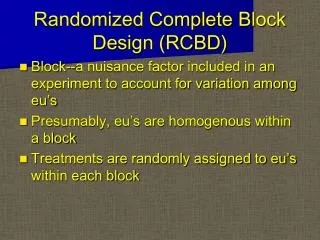
2. Randomized Complete Block Design The experimental units are allocated to groups, or blocks, in such a way that the experimental units within blocks are relatively homogenous and that the number of experimental units within a block is equal to the number of treatments being investigated The treatments are assigned at random to the experimental units within each block

3. Model The basic assumption for a randomized complete block design with one observation per experimental unit is that the observations may be represented mathematically by the linear statistical model yij =  + ai + j + ij , i = 1, 2, …, k j = 1, 2, …, b

4. Model where yij is the observation associated with the ith treatment and jth block,  is the true mean effect ai is the true effect of the ith treatment j is the true effect of the jth block ij is the experimental error and ij ~ N(0, s2)

5. Block Treatment 1 . . . j . . . b 1 y11 . . . y1j . . . y1b T1. y1. : i yi1 . . . yij . . . yib Ti. yi. : k yk1 . . . ykj . . . ykbTk. yb. TotalT.1 . . . T.j . . . T.b T.. Meany.1. . . y.j . . . y.b y.. Statistical Layout Total Mean

6. Analysis of Variance In partitioning the total variation of the observations into the variation attributable to mean, treatments, and random error, the Sum-of-Squares is used: Total Sum of Squares = Treatment Sum of Squares + Block Sum of Squares + Error Sum of Squares SST = SSA + SSB + SSE

7. Analysis of Variance = treatment sum of squares = = sum of squares due to blocks = = error sum of squares = SST - SSA - SSB =

8. Analysis of Variance - Computational Formulas

9. Analysis of Variance Table Sources of Degrees of Sum of Mean of F- Variation Freedom Squares Squares Ratio Treatments k - 1 SSA Blocks b - 1 SSB Experimental Error (b - 1)(k - 1) SSE Total bk-1 SST

10. Example Data were collected from a sample of 30 wafers. For each wafer, the thickness of the wafers on positions 1 and 2 (outer circle), 18 and 19 (middle circle) and 28 (inter circle) were measured.

11. Example – Solution Block Treatment 1 2 3 . . . 30 1 240 238 239 . . . 2417213 240.43 2 243 242 242 . . . 243 7273 242.43 18 250 245 246 . . . 2497382246.07 19 253 251 250 . . . 255 7473 249.10 28 248 247 248 . . . 2537412247.07 Total1234 1223 1225 . . . 1241 36753 Mean246.8 244.6 245 . . . 248.2245.02 Total Mean

12. Example – Solution overallaverage=245.02

13. Example Solution Continued overallaverage=245.02

14. Analysis of Variance Table Sources of Degrees of Sum of Mean of F- Variation Freedom Squares Squares Ratio Treatments 29 601.5 Block 4 1417.733 Experimental Error 116 406.2667 Total 149 2425.5

15. Example When using the 0.05 level of significance to test for differences among the positions, the decision rule is to reject the null hypotheses if the calculated F value exceeds 2.45, the upper-tailed critical value from the F distribution with 4 and 116 degrees of freedom in the numerator and denominator, respectively. Because F=101.20> Fu=2.45, we reject H0 and conclude that there is evidence of a difference in the average thickness for the different positions. As a check on the effectiveness of blocking, we reject H0 because F=5.922 > Fu=1.57. From this we conclude that there is evidence of difference among the wafers and that blocking has been advantageous.