Sensitivity Analysis of Mesoscale Forecasts from Large Ensembles

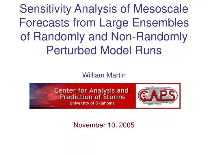
1. Sensitivity Analysis of Mesoscale Forecasts from Large Ensembles of Randomly and Non-Randomly Perturbed Model RunsWilliam MartinNovember 10, 2005

2. Sensitivity Analysis Has a Number of Uses: -- Identifying physical connections -- Data assimilation -- Targeting observations -- Weather modification

3. ADJOINTS For determining the sensitivity field of a forecast to conditions at an earlier time, the use of the adjoint of a forward numerical model has, until recently, been the only method available. Adjoints are integral parts of 4-dimensional variational data assimilation systems (4DVAR) in which the model state is sought which minimizes the difference between the forecast and a set of observations. The sensitivity of model error to initial fields is determined by an adjoint calculation. This is then used in a minimization scheme.

4. Adjoints are easiest to understand in terms of the chain rule for differentiation applied recursively. • Consider, for example, the following implementation of the Lorenz model (1963):

5. Using simple first order time differencing, the forecast parameters of the Lorenz model over one time step are:

6. For a response function, J, we choose the total energy: • And we might be interested in the sensitivity of J to the initial conditions:

7. As J is defined at the forecast time, N, we start at that time with: • For the sensitivity of J to the model state at the previous time step, we invoke the chain rule:

8. In matrix notation this is: Or: And by recursion: Terms on RHS associate, but don’t commute

9. For the Lorenz model with 3 degrees of freedom, the adjoint is easy to code and implement. • For a complex mesoscale model with millions of degrees of freedom and thousands of lines of code, differentiation is difficult. • Also, calculating the adjoint requires storing the model state at every time step from the forward run.

10. As part of the IHOP (2002) program, we wanted to obtain the sensitivity of model forecasts of convective initiation. • Delays in having the adjoint of the ARPS (the Advanced Regional Prediction System) ready, led to an attempt to obtain this information using Very Large Ensembles (VLE) of forward model runs. • This is a brute-force way of solving the problem, with the brute being large parallel computing systems at PSC and NCSA.

11. The VLE method finds the sensitivity of J to some initial variable at some point in space by applying an initial perturbation at that point and in that variable. • The assembly of sensitivity fields requires the consideration of such perturbations at every location and in every variable. This is potentially a very large number of perturbations (the model configuration we use has over 6 million degrees of freedom). • Each perturbation needs a separate forward model run.

12. Model Configuration • ARPS model with numerous physical paramemterizations • 135X135X53 grid points ~ 1 million grid points • DX=DY=9 km

13. Initial fields used for the ARPS model run 10-m water vapor 10-m wind barbs

14. 6-hour forecast fields 10-m wind barbs 10-m water vapor

15. Forecast Precipitation Fields Total accumulated ppt Vertically integrated liquid

16. In order to reduce the number of perturbations, the horizontal domain is divided into 45 X 45 tiles (3 grid points by 3 grid points). • Sensitivity to boundary layer fields can then be found if we use perturbations 1 km deep at the surface at each of these tiles. • 45 X 45 perturbations + 1 unperturbed run =2026 perturbed model runs to make. • This runs in parallel in about 7 hours.

17. Sample Initial Perturbation 1 g/kg perturbation in a patch 27X27X1 km

18. Backward sensitivities at an (x,y) location are calculated as the change in response function value (unperturbed minus perturbed) divided by the initial perturbation size at that location. This approximates The exact sensitivity if the perturbations are small enough:

19. Non-Dimensional Sensitivity With J0=unperturbed run value And a0=unperturbed field value

20. Sensitivity of forecast Qv in box to initial boundary layer Qv perturbations After 6 hours: dryline Effects of diffusion spread over time Which combines with advection No rain in this region

21. Forward- and Backward-in-Time Sensitivities dryline Forward in time Backward in time

22. Sensitivity of Total Rain Along the Dryline to ABL Water Vapor Perturbations -1 g/kg perturbations +1 g/kg perturbations

23. Sensitivity of Rain Along the Cold Front to Initial ABL Moisture +1 g/kg perturbations -1 g/kg perturbations

24. Strong Non-Linear Sensitivity Near Cold Front led to 3 cm precip here Control run Initial perturbation here

25. Strong Non-Linear Sensitivity Near Cold Front led to 12 cm precip here Control run Initial perturbation here

26. Perturbing more than one initial variable simultaneously does not ordinarily work as the effects of two separate perturbations interfere with each other, and there is no way to undo the combined effects in the forecasts. • However, if a large number of randomly perturbed runs is attempted, then statistics may be applied. • This is similar to the method of calculating error covariances using the Ensemble Kalman Filter.

27. If you have N forecasts in which every variable has a random perturbation, then you obtain N different values for the response function, J. • To determine the sensitivity of the forecast to an initial value of some field at some point in space, these N J values can be linearly regressed against the N random (but known) perturbations of that variable.

28. Slope of best fit line provides J Delta X

29. For this test, we used binary perturbations; that is, the perturbations were either plus or minus some fixed value, say, 1 K of temperature. Whether the value is to be + or – 1 K is chosen at random. • The RANDOM_NUMBER function of FORTRAN90 is used, which may not be good enough.

30. Far more negative perturbations Than positive perturbations

31. Sensitivity of Potential Temperature in Box to initial Potential Temperature Perturbations Random VLE 400 runs 2026 runs Max=.0021 MAX=.0020

32. Sensitivity of Total PPT in the Box to Initial Boundary Layer Potential Temperature VLE Random 2026 model runs 400 model runs Max=5.2 Max=5.4

33. Log-log plot of RMS noise of a sensitivity field versus ensemble size

34. Theoretically, noise should scale with the square root of the ensemble size. O=theoretical noise reduction

35. Summary • Both the VLE and random perturbation techniques work well and produce similar results. • They are viable alternatives to an adjoint, but do require considerable computing resources. • Using forward model runs can give different information than an adjoint because an adjoint provides the exact sensitivity to a infinitesimal perturbation, while a perturbation method provides the actual impact of a finite perturbation. • The random perturbation method requires potentially fewer forward model runs, but the reduction of noise to an acceptable level may still require a large ensemble.