Calibration of Distributed Hydrology-Soils-Vegetation Model to Lake Whatcom Watershed, Washington State

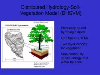
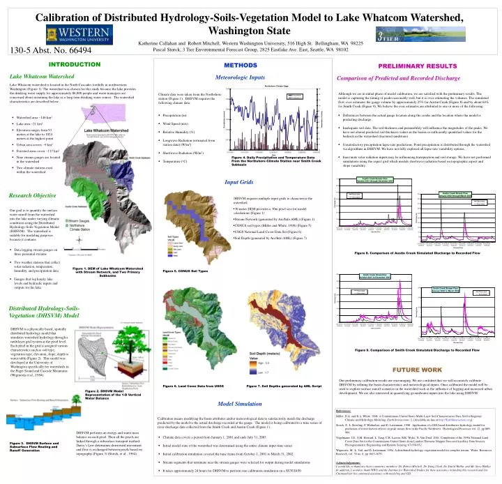
1. Calibration of Distributed Hydrology-Soils-Vegetation Model to Lake Whatcom Watershed, Washington State Katherine Callahan and Robert Mitchell, Western Washington University, 516 High St. Bellingham, WA 98225 Pascal Storck, 3 Tier Environmental Forecast Group, 2825 Eastlake Ave. East, Seattle, WA 98102 130-5 Abst. No. 66494 INTRODUCTION METHODS PRELIMINARY RESULTS Lake Whatcom Watershed Meteorologic Inputs Comparison of Predicted and Recorded Discharge Lake Whatcom watershed is located in the North Cascades foothills in northwestern Washington (Figure 1). The watershed was chosen for this study because the lake provides the drinking water supply for approximately 86,000 people and water managers are concerned about sustaining the lake as a long term drinking water source. The watershed characteristics are described below. Although we are in initial phase of model calibration, we are satisfied with the preliminary results. The model is capturing the timing of peaks reasonably well, but it is over estimating the volumes. The simulated flow over estimates the gauge volume by approximately 25% for Austin Creek (Figure 8) and by about 64% for Smith Creek (Figure 9). We believe the over estimates are attributed to one or more of the following: Climate data were taken from the Northshore station (Figure 1). DHSVM requires the following climate data: • Precipitation (m) • Wind Speed (m/s) • Relative Humidity (%) • Longwave Radiation (estimated from station data) (W/m2) • Shortwave Radiation (W/m2) • Temperature (oC) • Differences between the actual gauge location along the creeks and the location where the model is predicting discharge. • Inadequate soil data. The soil thickness and permeability will influence the magnitudes of the peaks. We have not altered predicted soil thickness values in the basins or sufficiently quantified values for the bedrock in the watershed (fractured sandstone). • Unsatisfactory precipitation lapse rate predictions. Point precipitation is distributed through the watershed via algorithms in DHSVM. We have not fully explored all lapse rate variability options. • Inaccurate solar radiation inputs may be influencing transpiration and soil storage. We have not performed simulations using the aspect grid which models shortwave radiation based on topographic aspect and slope variability. • Watershed area ~146 km2 • Lake area ~21 km2 • Elevation ranges from 93 meters at the lake to 1024 meters at the highest point • Urban area covers ~9 km2 • Forested areas cover ~117 km2 • Nine stream gauges are located in the watershed • Two climate stations exist within the watershed Figure 4. Daily Precipitation and Temperature Data From the Northshore Climate Station near Smith Creek Subbasin Input Grids Research Objective DHSVM requires multiple input grids to characterize the watershed. • 30 meter DEM provides a 30m pixel size for model calculations (Figure 1) • Stream Network (generated by Arc/Info AML) (Figure 1) • CONUS soil types (Miller and White, 1998) (Figure 5) • USGS National Land Cover Data Set (Figure 6) • Soil Depth (generated by Arc/Info AML) (Figure 7) Our goal is to quantify the surface water runoff from the watershed into the lake under varying climatic conditions using the Distributed Hydrology-Soils-Vegetation Model (DHSVM). The watershed is suitable for modeling purposes because it contains • Data logging stream gauges on three perennial streams • Two weather stations that collect solar radiation, temperature, humidity, and precipitation data • Gauges that log hourly lake levels and hydraulic inputs and outputs for the lake Figure 8. Comparison of Austin Creek Simulated Discharge to Recorded Flow Figure 1. DEM of Lake Whatcom Watershed with Stream Network, and Two Primary Subbasins Figure 5. CONUS Soil Types Distributed Hydrology-Soils-Vegetation (DHSVM) Model DHSVM is a physically based, spatially distributed hydrology model that simulates watershed hydrology through a multilayer grid system at the pixel level. Each pixel in the grid is assigned various characteristics such as soil type, vegetation type, elevation, slope, depth to water table (Figure 2). This model was developed at the University of Washington specifically for watersheds in the Puget Sound and Cascade Mountains (Wigmosta et al., 1994). Figure 9. Comparison of Smith Creek Simulated Discharge to Recorded Flow FUTURE WORK Our preliminary calibration results are encouraging. We are confident that we will accurately calibrate DHSVM by refining the basin characteristics and meteorological inputs. Once calibrated the model will be used to explore surface runoff scenarios in the watershed such as the influence of logging and increased urban development. We are also interested in quantifying groundwater inputs into the lake using DHSVM. Figure 6. Land Cover Data from USGS Figure 7. Soil Depths generated by AML Script Figure 2. DHSVM Model Representation of the 1-D Vertical Water Balance Model Simulation References: Miller, D.A. and R.A. White, 1998: A Conterminous United States Multi-Layer Soil Characteristics Data Set for Regional Climate and Hydrology Modeling. Earth Interactions, 2. [Available on-line at http://EarthInteractions.org] Storck, P., L. Bowling, P. Wetherbee, and D. Lettenmair, 1998. Application of a GIS-based distributive hydrology model for prediction of forest harvest effects on peak stream flow in the Pacific Northwest. Hydrological Processes vol. 12, pp 889- 904. Vogelmann, J.E., S.M. Howard, L. Yang, C.R. Larson, B.K. Wylie, N. Van Driel, 2001. Completion of the 1990s National Land Cover Data Set for the Conterminous United States from Landsat Thematic Mapper Data and Ancillary Data Sources, Photogrammetric Engineering and Remote Sensing, 67:650-652. Wigmosta, M., L. Vail, and D. Lettenmair, 1994. A distributed hydrology-vegetation model for complex terrain. Water Resources Research, vol. 30 no. 6, pp 1665-1679. Acknowledgements: I would like to thank my thesis committee members: Dr. Robert Mitchell, Dr. Doug Clark, Dr. David Wallin, and Mr. Steve Walker. In addition, I would to thank WWU and the Institute for Watershed Studies for their assistance in funding this research and Jay Chennault for his continued assistance with modeling and GIS. Calibration means modifying the basin attributes and/or meteorological data to satisfactorily match the discharge predicted by the model to the actual discharge recorded at the gauge. The model is being calibrated to a time series of river-discharge data collected from the Smith Creek and Austin Creek (Figure 1). DHSVM performs an energy and water mass balance on each pixel. Then all the pixels are linked through a subsurface transport method: Darcy’s Law determines downward movement and flow is exchanged between pixels based on topography (Figure 3) (Storck, et al., 1994). • Climate data covers a period from January 1, 2001 and ends July 31, 2003 • Initial model state of the watershed was determined using the entire climate input-time series • Initial calibration simulation covered the time frame from October 1, 2001 to March 31, 2002 • Stream segments that terminate near the stream gauges were selected for output during model simulations • It takes approximately 24 hours for DHSVM to perform one calibration simulation on a SUN E450 Figure 3. DHSVM Surface and Subsurface Flow Routing and Runoff Generation