Download
1 / 30
360 likes | 503 Views
Measures of Dispersion. Measures of Dispersion – measures that help us learn about the spread of a data set Together, with measures of central tendency, give a better picture of a data set than either one alone. Range. What’s the range of this data set?

E N D
Measures of Dispersion – measures that help us learn about the spread of a data set Together, with measures of central tendency, give a better picture of a data set than either one alone.
Range What’s the range of this data set? What are some disadvantages of the range?
Disadvantages - Like the mean, the range is heavily influenced by outliers, therefore, not a good measure of dispersion of data with outliers. In the previous example, if the outlier is removed and the range is recalculated, the range becomes 20,252 square miles. • Also, the range only uses 2 values, largest and smallest, leaving all the numbers in the middle ignored. Range can be useful, but not the best measure of dispersion.
Standard Deviation Standard deviation – this value tells us how close the values of a data set are clustered around the mean. Most commonly used measure of dispersion. Low value vs. high value of standard deviation The lower the standard deviation, the data set values are spread over a smaller range around the mean. The higher the standard deviation, the data set values are spread over a larger range around the mean.
Variance Standard deviation is found by taking the positive square root of the variance. Formulas for variance: read “sigma squared”, is the population variance is the sample variance Consequently, standard deviation for the population is , And standard deviation for a sample is .
The or is known as the deviation of the x value from the mean. What should the sum of the deviations always equal. The sum of these deviations is always zero. That is, and
Example: Given the following four test scores 82, 95, 67, and 92, the mean would be The deviations would be calculated as Since the sum of the deviations always equals zero, we square the deviations to calculate both variance and standard deviation, giving us
Calculating Variance and Standard Deviation by hand Find the mean: so using the variance formula:
Short cut formula (?) Variance = 257.72 Take the square root for the standard deviation or $16.05 billion
On the calculator Press “stat” Then scroll to the right one space Then enter and enter again Do you want “s” for sample or for population Press “stat” then enter Type in the list of numbers
Observation The values of the variance and the standard deviation are never negative. Why? Can it be zero? When? The variance and standard deviation is zero when there is no variation, but never negative.
You do another example Given the earnings (in thousands) before taxes for all six employees of a small company 48.50 38.40 65.50 22.60 79.80 54.60 Find the range, variance, and standard deviation. Range = 79.80 – 22.60 = 57.20 Variance = 337.0489 Standard deviation = $18.359 thousand or $18,359
Exit questions • What are the 3 measures of dispersion? • Can the variance have a negative number? Can the standard deviation have a negative number? • When is the value of the standard deviation for a data set zero? • The following data set belongs to a population: 5 -7 2 0 -9 16 10 7 Calculate the range, variance, and standard deviation.
Normal Curve Normal Curve – bell shaped and symmetrical median, and mode are all the middle value
Using the Empirical Rule The age distribution of a sample of 5000 persons is bell-shaped with a mean of 40 years and a standard deviation of 12 years. Determine the approximate percentage of people who are 16 to 64 years old.
16 is 2 standard deviations to the left of the mean which is 47.5% 64 is 2 standard deviations to the right of the mean which is another 47.5% Therefore, there are , or of the people are between the ages of 16 and 64. 68% lie within + or – 1 standard deviation 95% lie within + or – 2 standard deviations 99.7% lie within + or – 3 standard deviations The Empirical Rule
Practice A large population has a mean of 310 and a standard deviation of 37. • What percentage of the observations fall in the interval ? • What are the values at ? • What percentage fall between 273 and 384?
Exit questions • The prices of all college textbooks follow a bell-shaped distribution with a mean of $105 and a standard deviation of $20. • A. Using the empirical rule, find find the percentage of all college textbooks with their prices between $85 and $125. • Using the empirical rule, find the interval that contains the prices of 99.7% of college textbooks.
Quartiles Quartiles – 3 summary measures that divide a ranked data set into 4 equal parts. The second quartile, , is also know as the median. The first quartile, , is the middle value of the observations less than the median. The third quartile, , is the middle value of the observations more than the median. • Values less than the median Values greater than the median • 24 28 33 33 37 39 47 51 59 • 30.5 the median 49
Interquartile Therefore, for the data 24 28 33 33 37 39 47 51 59 Interquartile is the range between the first and third quartiles. Interquartile range = The IQR of this range is
Percentile rank is the 25th % - that is 25% of all data is less than and 75% of all data is greater than is the 75th % - 75% of all data is less than and 25% of all data is greater than Median (or ) is the 50th % - 50% of data is less than median, and 50% greater than the median
Constructing Box and Whisker plots Given the income (in thousands) for a sample of 12 households: 35 29 44 72 34 64 41 50 54 104 39 58 Construct a box and whisker plot Find 29 34 35 39 41 44 50 54 58 64 72 104 Median Also need: Minimum = 29 Maximum = 104 IQR = 61 – 37 = 24
5 number summary: 29, 37, 47, 61, 104 Median 85 95 105 75 55 65 45 25 35
Practice • Prepare a box and whisker plot for the following data: 15 9 12 11 7 6 9 10 14 3 6 5 3 5 6 6 7 9 9 10 11 12 14 15 Median = 9 = 6 = 11.5 Min = 3 Max = 15 12 14 16 10 6 8 4 0 2
Using quartiles to determine outliers Formula for finding “inner fences”: Find the values that are 36 : 37 - 36 = 1 : 61 + 36 = 97 Any values below 1 or above 97 can be considered outliers.
Exit question: • The following data give the time (in minutes) that each of 20 students waited in line at their bookstore to pay for their textbooks. 15 8 23 21 5 17 31 22 34 6 5 10 14 17 16 25 30 3 31 19 Prepare a box and whisker plot