Download
1 / 34
340 likes | 472 Views
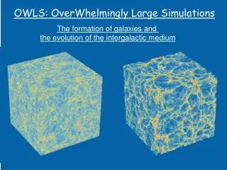
The formation of galaxies and the evolution of the intergalactic medium. OWLS: OverWhelmingly Large Simulations. Joop Schaye, Craig Booth, Claudio Dalla Vecchia, Alan Duffy, Marcel Haas, Volker Springel, Tom Theuns, Luca Tornatore, Rob Wiersma, …. Outline.

E N D
The formation of galaxies and the evolution of the intergalactic medium OWLS: OverWhelmingly Large Simulations Joop Schaye, Craig Booth, Claudio Dalla Vecchia, Alan Duffy, Marcel Haas, Volker Springel, Tom Theuns, Luca Tornatore, Rob Wiersma, …
Outline 1. Introducing cosmological simulations and OWLS 2. Preparing for and coping with lots of data 3. Data format and units 4. Microsimulations 5. Virtual observations of simulations 6. Discussion points
Example science questions • What determines the SF history of the universe? • Where are the baryons and how can they be detected? • Where are the metals and how can they be detected? • How does galaxy formation depend on environment? • What are the large-scale effects of galactic winds driven by stars and AGN? • Virtual observations
Cosmological hydro simulations • Evolution from z>~100 to z ~< 10 of a representative part of the universe • Boundary conditions: periodic • Expansion solved analytically and scaled out • Initial conditions from the CMB • Components: cold dark matter, gas, stars, radiation (optically thin) • Scales ~< kpc to ~ 100 Mpc • Sub-grid modules are a crucial part of the game • Discretizaton: time and mass (SPH)
The OWLS simulations • LOFAR IBM Bluegene/L (12k CPUs, PowerPC 440, 700 MHz, 500 MB per 2 CPUs) • Cosmological (default: WMAP3) • Hydrodynamical (SPH) • Gadget III • 2xN3 particles, N = 512 for most • Two sets: • L = 25 Mpc/h to z=2 • L = 100 Mpc/h to z=0 • Runs repeated many times with varying physics/numerics • Status: runs nearly done, starting analysis
OWLS subgrid physics improvements • New star formation • New wind model • Added chemodynamics • New cooling
OWLS Numerical Resolution • 25 Mpc/h (run to z=2): • m_bar = 1x10^6 Msun/h • Softening = 2 kpc/h comoving < 0.5 kpc/h proper • 100 Mpc/h (run to z=0): • m_bar = 7x10^7 Msun/h • Softening = 8 kpc/h comoving < 2.0 kpc/h proper
Zoom CDV, OWLS project
Outline 1. Introducing cosmological simulations and OWLS 2. Preparing for and coping with lots of data 3. Data format and units 4. Microsimulations 5. Virtual observations of simulations 6. Discussion points
OWLS data volume • 7 - 42 floats per particle up to 168 bytes/particle • 268 M particles per snapshot 26 GB/snapshot • Up to 35 snapshots per simulations 900 GB/simulation • ~60 large simulations 54 TB of snapshot data
How do we analyze 50+ TB of data? • First analyze lower resolution versions • Use hdf5 only read what is actually needed • Use fast visualization software (e.g. avoid SPH interpolation) • Produce as much as possible on the fly: • Logs (e.g. SF histories) • Grids (e.g. baryon distribution) • Sight lines (e.g. QSO absorption spectra) • Images (e.g. for videos) • Zooms saved on the fly (e.g. most massive object) • Diagnostic particle arrays (e.g. max temperature) • Group catalogues
Analysis that can be done on a notebook: • Low-resolution versions • Evolution of globally averaged (or gridded) quantities • Halo integrated properties • Halo profiles • Absorption spectra • Most things related to zooms
Outline 1. Introducing cosmological simulations and OWLS 2. Preparing for and coping with lots of data 3. Data format and units 4. Microsimulations 5. Virtual observations of simulations 6. Discussion points
Hdf5 – Hierarchical Data Format • Binary fast I/O and compressed • Machine-independent • Intuitive hierarchical “directory-like” structure • Individual elements can be read, modified and saved • Easy to add meta-data • Utilities available to view the data in ascii or graphical form (incl. tables, images) • Very easy to read/write from IDL, C, F90 • Free
Data format: Units • Data should use code units to allow easy debugging, restarting • But data should be in physically sensible units to allow analysis by external users • Cosmological data should clarify h and aexp dependence for external users Solution: use code units but include conversion factors to cgs and aexp and h dependencies as meta-data.
Outline 1. Introducing cosmological simulations and OWLS 2. Preparing for and coping with lots of data 3. Data format and units 4. Microsimulations 5. Virtual observations of simulations 6. Discussion points
Outline 1. Introducing cosmological simulations and OWLS 2. Preparing for and coping with lots of data 3. Data format and units 4. Microsimulations 5. Virtual observations of simulations 6. Discussion points
Virtual Observations: Uses • Guide the design of observational campaigns and instruments • Test data analysis pipelines • Determine selection effects • Test theoretical models • PR/education
Virtual Observations: Types • Galaxy magnitudes • Population synthesis, which depends on • Assumed IMF • Age and composition of star particle • Dust column and assumed reddening law • Stellar light images • Absorption spectra • Gas emission maps (2-D: images, 3-D: IFU datacubes) • Other maps: e.g. lensing, SZ, dust absorption/emission
Creating Virtual Observations • Compute emission and/or absorption of each resolution element • Project and grid data, optionally combine different time slices (e.g. lightcones) • Observe with chosen instrument (easiest step)
Virtual Observations – Star light • Population synthesis • Save initial mass, age, and composition of individual star particles • Assume IMF • Dust column • Save mass and composition of individual gas particles • Assume reddening law • Require fast calculation of SPH column densities
Virtual Observations – Gas absorption • Require gas mass, position, velocity, density, temperature, composition • Assume ionization equilibrium and use ionization balance tables (e.g. CLOUDY) • Collisional ionization temperature • Photo-ionization density, temperature, radiation field
Virtual Observations – Gas emission • Require gas mass, position, density, temperature, composition, (velocity) • Assume ionization equilibrium and use emissivity tables (e.g. CLOUDY) • Dust columns
On-demand Virtual Observations of cosmological simulations • Computed from physical properties (e.g. gas density, temperature) • Computed from pre-calculated “ideal” observables • Example: narrow band gas emission for various assumed radiation fields, chemical compositions, or density/temperature cuts • Allows one to vary both physical assumptions and instrumental characteristics • Computationally expensive • Example: narrow band gas emission for a fixed radiation field and chemical composition • Cannot vary physical assumptions • Relatively cheap
VOs from physical properties • Challenge: Analysis of 3-D simulations is typically memory-intensive (512^3 1 single precision array is 0.5 GB) • Solution: • Prepare data with reduced dimensionality, calculate on demand • 1-D: Absorption spectra, dust columns • 2-D: Images from integrated quantities • Problem: Emission & (gas) absorption depends on local 3-D rather than projected 2-D properties
On-demand VOs • Feasible now or in the near future: • (VOs based on) object catalogues • Absorption spectra • SZ effect • Images of stellar light (though maybe not full lightcones) • Other VOs from pre-calculated observables
Discussion points: • Are raw cosmological simulation data sets too large to put in the VO? • Is there a place for non-VO, processed data products in the VO? (e.g. physical properties) • Must VO software for non-simulators be like a black box? • Is it desirable to create black boxes for non-simulators? • How to prevent wasting of resources by wrong use of VO software?