Download
1 / 19
190 likes | 347 Views
Computational Statistics. Multiple linEAr regression. Basic ideas. Predict values that are hard to measure irl, by using co-variables (other properties from the same measurement in a sample population) We will often consider two (or more) variables simultaneously.

E N D
Computational Statistics Multiple linEAr regression
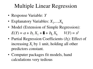
Basic ideas • Predict values that are hard to measure irl, by using co-variables (other properties from the same measurement in a sample population) • We will often consider two (or more) variables simultaneously. • 1) The data (x1, y1),…, (xn, yn) are considered as independent replications of a pair of random variables, (X, Y ). (observational studies) • 2) The data are described by a linear regression model (planned experiments) • yi = a + b * xi + εi; i = 1, ... , n
The linear model • Multiple regression model • Predicts a response variable using a linear function made up of co-variables (predictor variables) • Goal: • to estimatetheunknown parameter (βp) ofeachcovariable (Xp) (itsweight/significance) • to estimatethetheerrorvariance • Ŷ = b1 + b2 * X1 + b3 * X2 +…. + ε • ε = systematicerros + randomerrors
The linear model II • Quantify uncertainty in empirical data • Assignsignificance to variouscomponents (covariables) • Find a good compromise between between model size and the ability to describe data (and hence the response)
The linear model III • Sample size n > numberofpredictors p • p columnvectorsarelinerarly independent • errorsarerandom=> responsesarerandom as well • E(ε) = 0. Ifε ≠ 0 => systematic error, if the model is correct
Modelvariations • Linear regression throughtheorigin • p1 = 1, Ŷ = B1 x X + ε • Simple linear regression • p1 = 2, Ŷ = B1 + B2 x X + ε • Quadratic regression • p1 = 3, Ŷ = B1 + B2 x X + B2 x X 2 + ε • Regression withtransformedpredictor variables (example) • Ŷ = B1 + B2 x log(X) + B2 x sin(X)+ ε • Data needs to be checked for linearity to identify model changes
Goals of analysis • A good fit with small errors using the method of least squares • Good parameter estimates – how much predictor variables explains (contributes to) the response in the chosen model • Good prediction of the response as a function of predictor variables • Using confidence intervals and statistical tests to help us reach these goals • Find the best model in an interactive process. Probably using heuristics
Least Squares • residual r = Ŷ(beta, covariates) – X (empirical) • Best βwhen r² is minimal for the chosen set of covariates (in the given model) • Least squares based on random errors => least squares are random too => different betas for each measured sample => different regression lines (Although, The Central Limit Theory predicts a “true” regression line with “enough” samples)
Linear Model Assumptions • E(error) = 0 (Linear equation is correct) • All xi’s are exact (no systematic error) • Error variance is constant (homoscedasticity). Empirical error variance = teoretical variance. • Otherwise weighted least squares can be used • Uncorrelated errors; Cov(ei, ej) = 0 for all i≠j. • Otherwise, generalized least squares can be used • Errors are normally distributed => Y normally distributed. • Otherwise, robust methods can be used instead of least squares
Model cautions • covariate problem (time-based) • Dangerous to use a fitted model to extrapolate where no predictor variables have been observed • Is the average height of the Vikings just a few centimeters?
Test and Confidence (any predictor) • Test predictor (p) using the null-hypothesis H0,p : βp = 0 againt the alternative Ha,p : βp ≠ 0 • Using t-test and P-values to determine the relevance • Quantifies the effect of the p’th predictor variable after having subtracted the linear effect of all other predictor variables on Y • Problem: All predictors might have significance due to correlation among predictor variables
Test and Confidence (global) • Using ANOVA (ANalysis Of VAriance) to test the hypothesis (H0) that all βs = 0 (no relevance) versus at least one β≠0 (Ha) • F-test to quantify the statistical significance of the predictor variables • Describe fitness using sum of squaresR2= SS(explained) / SS(total) = (Ŷ-E(Y)) 2 / ( Y-E(Y) ) 2
Tukey-Anscombe plot (linearity assumption) • Using residuals as an approximation of the unobservable error and linearity • Plotting residuals against the fitted values (response) • Correlation should be zero -> random fluctuation of values around a horisontal through zero line • A trend-plot is evidence of a non-linear relation (or systematic error) • Possible solution : transform the response variable or perform a weighted regression • SD grows : Y -> log(Y) • SD grows as square root : Y->SQRT(Y)
The Normal/QQ Plot (norm.distr.assumptions) • Checking the normal distribution using quantile-quantile plot (qqplot) or normal plot • y-axis = Quantiles of the residuales,x-axis = theoretical quantiles of N(0,1) • Normal plot gives a straight line intercepting the mean with a slope value = standard deviation
Model selection • We want the model to be as simple as possible • What predictors should be included? • We want the best/optimal model, not necessarily the true model • More predictors -> higher variance • Optimize the bias-variance trade-off
Searching for the best model • Forward selection • Start with the smallest model, include the predictor which reduces the residual sum of squares most until a large number of predictors have be selected. Choose the model with the smallest Cp-statistic • Backward selection • Start with the full model, Exclude the predictor which increases the residual sum of squares the least until all, or most, predictor variables have been deleted. Choose the model with the smallest Cp-statistic • The cross-validated R2 can be used to calculate the best model when multiple models have been identified (using forward or backward selection)