Download
1 / 4
40 likes | 124 Views
Proposing a DMT monitor for studying micro-seismic noise and up-conversions. S. Mukherjee & R. Grosso UTB & U. Erlangen, Germany. LSC Det Char Telecon, 05/18/07. Motivation. NoiseFloorMon has been running since the onset of S5. This monitor looks for non-stationarities

E N D
Proposing a DMT monitor for studying micro-seismic noise and up-conversions S. Mukherjee & R. Grosso UTB & U. Erlangen, Germany LSC Det Char Telecon, 05/18/07
Motivation NoiseFloorMon has been running since the onset of S5. This monitor looks for non-stationarities in 4 frequency bands – 0-16, 16-32, 32-64 and 64-128 Hz. This monitor looks at the cross-correlations with the seismic channels and reports the 10 loudest events everyday. These events are analyzed in the time-frequency domain and also looked at using Q-scan and BN event displays. (Graduate student R. Stone is working on the off-line analysis). Following discussions with Robert Schofield, we have come up with the idea of using the same median based statistics as used in the NoiseFloorMon to analyze the noise seen in micro-seismic bands and the possible up-conversions. It is thus proposed that we write a new monitor that will look at specific frequency bands of interest and will correlate them with the higher frequencies to look for up-conversions. The following slides give the details of the frequency bands, why we choose them and the physical questions that we want to answer.
Bands to be analyzed (in Hz) 0.03 – 0.1 : Distant earthquake 0.1 – 0.3 : Micro-seismic peak 0.7 – 0.8 Large optic pendulum 0.9 – 1.1 Small optic pendulum 1.1 – 1.3 : BSC H-H mode 2.1 – 2.3 : BSC H-H mode 5.0 – 7.0 : BSC H-H mode 9.0 – 11.0 : BSC modes 11.5 – 12.5 : Optic bounce modes 15.0 – 17.0 : Mystery bounce modes 17.0 – 19.0 : Optic roll mode 19.0 – 20.0 : Motors (6 poles) 28.0 – 30.0 : Motors (4 poles) The median based estimate Of the noise floor variation Of these bands are to be correlated to that in the 80-100 Hz band. Coil current to be used instead of the seismic channels.
Output • The channels to be analyzed are : DARM-ERR, coil currents • (e.g. SUS-ETMY_COIL_LL) • Correlations will be studied between each of the low frequency bands and the 80-100 Hz band. • Output of the monitor will be a series of plots of peak correlation vs. time. • Large correlation epoch can be further analyzed in time domain and also using other existing tools.