Download
1 / 24
260 likes | 452 Views
L1 sparse reconstruction of sharp point set surfaces. HAIM AVRON, ANDREI SHARF, CHEN GREIF and DANIEL COHEN-OR. Index. 3d surface reconstruction Moving Least squares Moving away from least squares [l1 sparse recon] Reconstruction model Re-weighted l1 Results and discussions.

E N D
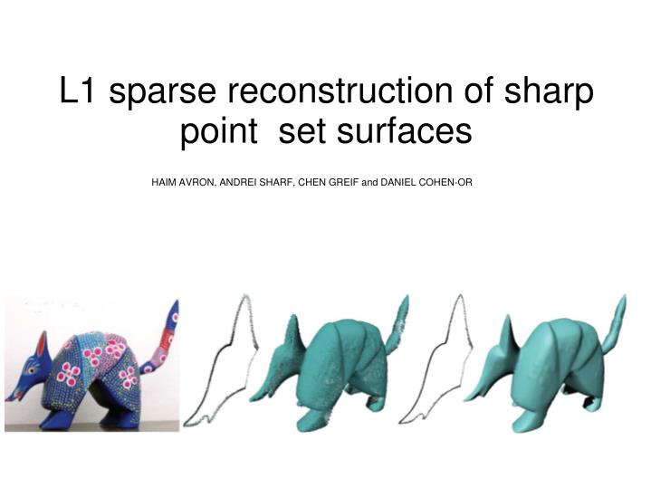
L1 sparse reconstruction of sharp point set surfaces HAIM AVRON, ANDREI SHARF, CHEN GREIF and DANIEL COHEN-OR
Index • 3d surface reconstruction • Moving Least squares • Moving away from least squares [l1 sparse recon] • Reconstruction model • Re-weighted l1 • Results and discussions
Moving least squares • Input: • Dense set of sample points that lie near a closed surface F with approximate surface normals. • [in practice the normals are obtained by local least squares fitting of a plane to the sample points in a neighborhood ] • Output : • Generate a surface passing near the sample points. • How does one do that : • Linear point function that represents the local shape of the surface near point s. • Combine these by a weighted average to produce a 3D function {I}, the surface is the zero implicit surface set of I. • How good is it ? • How close Is the function I to the signed distance function.
Total variation • The l1-sparsity paradigm has been applied successfully to image denoising and de-blurring using Total Variation (TV) methods • [Rudin 1987; Rudin et al. 1992; Chan et al. 2001; Levin et al. 2007] • Total variation utilizes the sparsity in variation of gradients in an image. • Dij is the discrete gradient operator , u is the scalar value • The corresponding term for gradient in a mesh is the normal of the simplex (triangle)
Reconstruction model • Error term : • Smooth surfaces have smoothly varying normals • Penalty function (error) defined on the normals • Total curvature Quadratic ; instead use • Pair wise normal difference l2 norm • Pi and pj are adjacent points pairwise penalty
Reweighted l1 • Consists of solving a sequence of weighted l1 minimization problems. • where the weights used for the next iteration are computed from the value of the current solution. • Each iteration solves a convex optimization, • The over all algorithm does not. • [Enhancing Sparsity by Reweighteed l1 Minimiaztion , Candes 2008]
Reweighted l1 • What is the key difference between l1 and l0 ? • Dependence on magnitude.
Geometric view error Minimize L2 –norm [sum of square errors] Minimize L1 norm [sum of differences] Minimize L0 norm [number of non zeros terms]
Orientation reconstruction • Orientation minimization consists of two terms • Global l1 minimization of orientation (normal) distances. • Constraining the solution to be close to the initial orientation.
Orientation reconstruction ctd • Orientation minimization consists of two terms • Global l1 minimization of orientation (normal) distances. • For a piece-wise smooth surface the set • Is sparse … why ? • Globally weighted l1 penalty function
Orientation reconstruction ctd • For a piece-wise smooth surface the set • Is sparse • Globally weighted l1 penalty function
Orientation reconstruction • Orientation minimization consists of two terms • Global l1 minimization of orientation (normal) distances. • Constraining the solution to be close to the initial orientation.
Geometric view error Minimize L2 –norm [sum of square errors] Minimize L1 norm [sum of differences] Minimize L0 norm [number of non zeros terms]
Criticisms Slow In reality the convex optimization although there are readily available solutions is a slow process. Results and Discussions • Advantages • Global frame work • Till now sharpness was a local concept
Discussions • A lot of room for improvement • Can I express this as a different form ? • Specially like the low rank and sparse error form we had before.