Download
1 / 10
100 likes | 357 Views
Lecture #23 EGR 261 – Signals and Systems. Read : Ch. 17 in Electric Circuits, 9 th Edition by Nilsson Ch. 7 in Linear Systems and Signals, 2 nd Edition by Lathi. Fourier Transform Properties

E N D
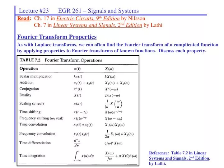
Lecture #23 EGR 261 – Signals and Systems Read: Ch. 17 in Electric Circuits, 9th Edition by Nilsson Ch. 7 in Linear Systems and Signals, 2nd Edition by Lathi Fourier Transform Properties As with Laplace transforms, we can often find the Fourier transform of a complicated function by applying properties to Fourier transforms of known functions. Discuss each property. Reference: Table 7.2 in Linear Systems and Signals, 2nd Edition, by Lathi.
Lecture #23 EGR 261 – Signals and Systems Table of Fourier Transforms In order to effectively use the Fourier transform properties just introduced, we must begin with a table of known Fourier transforms. Reference: Table 7.1 in Linear Systems and Signals, 2nd Edition, by Lathi.
Note that this is nearly identical to the time-shifting property using Laplace transforms: f(t - )u(t - ) ↔ F(s)e-s f(t) 10 t 10 16 Lecture #23 EGR 261 – Signals and Systems Time-shifting Property If f(t) ↔F(w) then f(t-) ↔ F(w)e-jw Note that e-jw is a complex number with magnitude of 1 and angle -w (recall that e-jw is written as 1-w in shorthand notation). So, Time shifting has no effect on |F(w)|, but shifts the phase by -w. Example: Find the Fourier transform of f(t) shown below. Hint: Note that this is shifted version of the function rect(t/).
Lecture #23 EGR 261 – Signals and Systems Example: Find the Fourier transform of f(t) = e-a|t- |. Sketch f(t), |F(w)|, and F(w) before and after time-shifting.
Lecture #23 EGR 261 – Signals and Systems Frequency-shifting (modulation) Property If f(t) ↔F(w) then Note: This property can be found by applying the duality property to the time-shifting property or easily proved using the definition of the Fourier Transform. f(t)ejwo ↔ F(w-wo) Note that since ejwot is a complex function, a practical application is to multiply a function by a real function, the sinusoid cos(wot), instead. Note: This property is the basis for amplitude modulation (AM radio). See the example on the left. If a signal, x(t) is multiplied by cos(wot), the carrier, then the amplitude of the x(t) is equal to the peak value of the modulated signal, x(t)cos(wot). The frequency spectrum of the signal is translated to the carrier frequency, wo. The original signal, x(t), can be retrieved from the modulated signal using an envelope detector. This is covered in depth in a communications course. Reference: Fig. 7.25 in Linear Systems and Signals, 2nd Edition, by Lathi.
f(t) 1 t -2 2 Lecture #23 EGR 261 – Signals and Systems • Example: For f(t) shown below: • Find and sketch F(w) • Sketch f1(t) = f(t)cos(10t) and F1(w) Example: Repeat the example above using some voice/music waveform and its corresponding spectrum. Assume that the carrier frequency is 850 kHz (AM 850)
Lecture #23 EGR 261 – Signals and Systems Time convolution property: If x(t) ↔ X(w) and h(t) ↔ H(w) then As we saw with Laplace transforms: Convolution in the time domain corresponds to multiplication in the frequency domain. We can find the convolution of two signals using: x(t)*h(t) ↔ X(w)H(w) x(t)*h(t) = F-1{X(w)H(w)} Frequency convolution property: If x(t) ↔ X(w) and h(t) ↔ H(w) then So, Multiplication in the time domain corresponds to convolution in the frequency domain (with a scale factor of (1/2π). x(t)h(t) ↔ (1/2π)X(w)*H(w)
h(t) y(t) = x(t)*h(t) x(t) Lecture #23 EGR 261 – Signals and Systems Circuit Analysis using Fourier Transforms Laplace transforms are used more commonly than Fourier transforms for circuit applications since: 1) the Laplace transform integral converges for a wider range of functions, and 2) Laplace transforms can be used to represent initial conditions in circuits. However, Fourier transforms can be used and work well with some functions that are not well-suited for Laplace transforms. Consider the circuit or system shown below: If an input x(t) is applied to the circuit or system, the output y(t) is: y(t) = x(t)*h(t). Taking the Fourier transform of both sides of the equation (and using the time-convolution property), we find that: Y(w) = X(w)H(w) Note that this is quite similar to our early use of Laplace transforms where Y(s) = X(s)H(s) Also note that
Lecture #23 EGR 261 – Signals and Systems Example(Problem 17.22 in Electric Circuits, by Nilsson) Find io(t) using Fourier transforms if vg = 36 sgn(t). Does the solution make sense? (Check initial and final values when the circuit is in steady state.)
Lecture #23 EGR 261 – Signals and Systems Example(Problem 17.29a in Electric Circuits, by Nilsson) Find io(t) using Fourier transforms if vg = 125cos(40,000t) V