Download
1 / 32
320 likes | 475 Views
Stratospheric and Mesospheric Applications of SCIAMACHY Limb Observations. 5th German SCIAMACHY Validation Team Meeting. C. von Savigny, A. Rozanov, G. Rohen, K.-U. Eichmann, E. J. Llewellyn * , J. W. Kaiser + , M. Sinnhuber, M. Scharringhausen, P. Ulasi, H. Bovensmann, and J. P. Burrows

E N D
Stratospheric and Mesospheric Applications of SCIAMACHY Limb Observations 5th German SCIAMACHY Validation Team Meeting C. von Savigny, A. Rozanov, G. Rohen, K.-U. Eichmann, E. J. Llewellyn*, J. W. Kaiser+, M. Sinnhuber, M. Scharringhausen, P. Ulasi, H. Bovensmann, and J. P. Burrows Institute of Environmental Physics/Remote Sensing, University of Bremen, Bremen, Germany * Department of Physics and Physics Engineering, University of Saskatchewan, Saskatoon, Canada + Remote Sensing Laboratories, University of Zurich, Zurich, Switzerland
Stratospheric applications Polar stratospheric clouds Minor constituent profiles Mesospheric applications Mesospheric ozone profiles OH* (3-1) rotational temperature retrievals Noctilucent clouds Outline
Illustration of the limb-scattering geometry SCIAMACHY Limb Geometry • Tangent height range: 0 to 100 km • Tangent height step size: 3.3 km • Vertical FOV: 2.6 km • Observation optimised for limb-nadir matching • Duration of Limb sequence: 60 s • Observed is limb scattered solar radiation and terrestrial airglow emissions • On the Earth’s night side limb emissions are observed in a dedicated mesosphere / thermosphere observation mode with tangent height between 75 and 150 km.
PSC detection with limb measurements Step I: Determine colour index profiles Step II: Determine vertical gradient of CI(TH): with TH = 3.3 km Theoretical maximum (TH) values for 15-30 km altitude range: a) 1.05 for pure Rayleigh atmosphere b) 1.1 for stratospheric background aerosol c) 1.16 for moderate volcanic aerosol d) 1.55 for extreme volcanic aerosol Detection threshold chosen:(TH) = 1.3 detection is somewhat biased towards optically thicker PSCs
PSC maps Maps of detected PSCs (open circles: detected PSCs) superimposed to UKMO temperature field at 550 K potential temperature (about 22 km) for August 7-12, 2003.
Temporal variation of PSC altitudes 190 190 195 190 190 195 195 195 No SCIAMACHY Observations No SCIAMACHY Observations No SCIAMACHY Observations PSC descent rates for 2003: Santacesaria et al. [2001] : 2.5 km / month at 66º S / 140º E based on a 9-year Lidar climatology Fromm et al. [1997] : 2.0 km / month derived from POAM II
The scia-arc website • The scia-arc website provides value-added scientific data products • Presently available limb data products: stratospheric profiles of O3, NO2 and BrO • In preparation: - mesospheric O3 profiles - maps of NLCs and PSCs - OH rotational temperatures at the mesopause http://www.iup.physik.uni-bremen.de/scia-arc
One week before the major stratospheric warming: September 12, 2002 Savigny et al. [2004]
At mid-latitudes typical BrO mixing ratios are about 10 pptv, corresponding to about 50 % of the available inorganic bromine (20 pptv). The rest is almost exclusively BrONO2 .[e.g., Sinnhuber et al., 2002] • Within the vortex BrO mixing ratios are most likely enhanced due to the reduced NO2, therefore reduced formation of BrONO2.
Retrieval of OH* (3-1) rotational temperatures • OH* produced and vibrationally-rotationally excited at mesopause altitudes by: • H + O3 OH* (v’ 9) + O2 + 3.3 eV • Airglow emission centered around 87 km with about 8 km FWHM • Relative population of rotational levels governed by Boltzmann’s distribution • Measurements of relative intensities of rotational emission lines makes • retrieval of OH rotational temperature possible • OH*(v’ = 3) is in local thermodynamical equilibrium (LTE) for lower rotational quantum numbers because: • - collisional frequency at 86 km is 3 104 s-1 • - lifetime of OH at v’ = 3 is about 0.014 s • rotational temperatures are equal to kinetic temperature of ambient air
R-branch Q-branch P-branch J = + 1 J = -1 J = 0 J’=5 Selection rule: J = 0,+1,-1 J’=4 ’=3 J’=3 J’=2 J’=1 J’=0 J’’=5 EJ J(J+1) J’’=4 ’’=1 Q-branch P-branch J’’=3 J’’=2 J’’=1 J’’=0
Sample OH spectral fit • Iterative retrieval approach: • linear fit with 2nd order polynomial • (2) non-linear fit (Levenberg-Marquard) • driving OH model, including -shift Impact of different Einstein coefficients used: Kovacs [1969], Mies [1974], Goldman et al. [1998] TKovacs – TMies = 1.1 K and TKovacs – TGoldman = 3.2 K
Coverage of Limb eclipse measurements Calibration measurements Limb measurements Calibration measurements Limb measurements Calibration measurements
SCIAMACHY Operations Change Request 19 • Replacement of nighttime Nadir observations by limb observations • Implemented on September 6, 2004
First validation results GRound-based Infrared P-branch Spectrometer (GRIPS) I at Hohenpeissenberg (47° N / 11° E) GRIPS-I data provided by Michael Bittner and Kathrin Höppner (DLR) Mesospheric Temperature Mapper (MTM) at Hawaii (21° N / 204° E) MTM data provided by Mike Taylor and Yucheng Zhao (Utah State University)
OH-Temperatures 2003 • Temperatures: • for latitudes from –20 to 70 deg • from July 2002 up to now.
Averaging kernels Weighting functions
Ozone depletion during the Oct. / Nov. 2003 SPEs HOx production by ionization: O2+ + O2 + M O2+•O2 + M O2+•O2 + H2O O2+•H2O + O2 O2+•H2O + H2O H3O+•OH + O2 H3O+•OH + H2O H3O+• H2O + OH H3O+• H2O + e- 2 H2O + H O2+ + H2O + e- O2 + H + OH (Courtesy M.-B. Kallenrode and M. Sinnhuber ) NOx is formed as well
Ozone depletion during the Oct. / Nov. 2003 SPEs • Ozone loss at 55 km and north of magnetic 60° N relative to October 20 – 24 reference period • 40 MeV protons penetrate the atmosphere Down to about 45 km altitude
Observations vs. Model Percent ozone loss north of 60° N magnetic latitude SCIAMACHY measurements Reference period: October 20 – 24, 2003 Model simulations (M. Sinnhuber)
Detection of Noctilucent Clouds (NLCs) UV limb radiance profiles with NLCs and without NLCs
NLC particle size determination I I.In single scattering approximation the PMC backscatter is given by: q(,): Differential scattering cross section S(): Solar irradiance spectrum II.The sun-normalized PMC backscatter spectrum: with spectral exponent
NLC particle size determination II The spectral exponent is related to the PMC particle sizes by Mie-calculations • Assumptions: • Mie theory, i.e., homogeneous dielectric • spheres • Refractive index of ice [Warren, 1984] • Log-normal distribution Simulated spectral exponents for log-normal distribution with = 1.4 Ambiguity:spectral exponent does not monotonically increase with increasing radius Use several and significantly different wavelengths to determine r and [von Cossart et al, 1999].
Conclusions • SCIAMACHY limb observations with their broad spectral coverage and extended altitude range both on the day and nightside allows a wide range of stratospheric and mesospheric to be studied: • Optically thin aerosols like NLCs and PSCs • Minor constituent profiles (O3, NO2, BrO; soon H2O, CH4) • Mesopause temperature (soon Rayeigh temperatures)