Download

1 / 25
250 likes | 263 Views
Basic Tools for General Equilibrium Analyses in Trade Model. Basic Tools for General Equilibrium Analysis. Good Y. Y. MU x. Y. MRS = - =. X. MU y. X. CI 0. Good X. Demand Side: Community Indifference Curve (CIC)

E N D
Basic Tools for General Equilibrium Analyses in Trade Model
Basic Tools for General Equilibrium Analysis Good Y Y MUx Y MRS = - = X MUy X CI0 Good X Demand Side: Community Indifference Curve (CIC) Shows various combinations of two goods with equivalent welfare Downward sloping And Convexity CI Since Y(MUy) = - X(MUx) -Y/X = MUx/MUy Diminishing marginal rate of substitution
Consumer demand is always satisfied with more goods Ordinal and Transitivity: Farther out from origin point Means higher welfare to consumer Good Y CI3 CI2 CI1 CI0 Good X
A = B = C = D CI1: A = D Good Y CI1 > CI0 D > C contradiction B A D CI1 C CI0 Good X Non-intersecting Community Indifference Curve CI0: B = A = C
These are the wrong Portions of CIC. Why? Good Y C0 Good X
Consumer equilibrium: Maximize welfare subject to the income constraint (Budget constraint) I2 Good Y y I1 A y1 CI0 x x1 0 Good X Slope of budget line: Y/X = (0y)/(-0x) = (I1/Py)/(-I1)Px) = - Px/Py = MRS At point A: (Px)(0x1) + (Py)(0y1) = I1 • y1 = (I1)/(Py) – (Px/Py)X1 • Y = (I1)/(Py) – (Px/Py)X Y/X = – Px/Py
Supply side: Production possibility frontier (PPF) Marginal rate of technical substitution Capital (K)x(MPPK) = - (L)x(MPPL) K/L = - MPPL/MPPK K/L= MRTS P’ K1’ K K1 P L Q1 L1 L1’ Labor 0 Isoquent concept: Show various combinations of two inputs that produce same level output Downward sloping and Convexity for possible substitution
Non-intersecting Farther out from origin point Means greater quantities of outputs Capital P’ K1’ Q4 K K1 P Q3 L Q2 Q1 L1 L1’ Labor 0
Constant return to scale: agiven percentage increase in all inputs will lead the same percentage increase in output Capital intensive output expansion path Capital G’ 4K1 Labor intensive output expansion path G P’ 2K1 Q2=20 K1 P Q1=10 L1 2L1 4L1 Labor 0
Producer Equilibrium:At the point the isoquant is tangent to the isocost. Firm maximizes output for the given cost (i.e., most efficient production), Or firm minimizes its factor cost for the given level of output. Capital K’ B2 P’ K B1 H K1 P Q2 Q1 0 L1 Labor L L’ The slope of isocost (or the factor price line) K/L = 0K/-0L = - (B1/r)/(B1/w) = w/r where r is labor wage, w is capital rental rate = MPPL/MPPK = MRTS At point P: B1 = rK + wL • rK = B1 – wL • K = (B1/r) – (w/r)L • K/L = - w/r
S-Isoquant (K/L)s K K Ks (K/L)c Kc Kc C-Isoquant Increasing K Increasing K Oc Oc Ls L L Increasing L Increasing L Lc Lc S is capital-intensive (K/L)s > (K/L)c or (L/K)s < (L/K)c C is labor-intensive (L/K)s < (L/K)c or (K/L)s > (K/L)c
Increasing L Ls Os K K Increasing K (K/L)c (K/L)c Kc Kc Ks Isoquant Increasing K Increasing K (K/L)s Oc Oc L L Increasing L Increasing L Lc Lc Resources allocation in two goods within a country
The Edgeworth Box: L 0s K Not Pareto Efficiency C5 C4 C3 V C2 C1 S5 S1 S2 S3 S4 K 0c L Contract curve: production efficiency locus with increasing opportunity cost
The Edgeworth Box: L 0s K C5 C4 C3 C2 Not Pareto Efficiency C1 V S1 S2 S3 S4 S5 K 0c L Contract curve: production efficiency locus with constant opportunity cost
Steel S0 S1 K2 C3 C2 S2 S3 C1 C0 Clothes L2 Country II: Capital abundant country
Steel S0 S1 C3 KI C2 S2 C1 S3 C0 Clothes LI Country I: Labor-abundant country
Constant vs. Increasing Opportunity Cost on the PPF Good Y PPF (or contract curve) with constant opportunity cost Increasing Opportunity Cost PPF (or contract curve) Decreasing increase Good X 0 Constant increase
General equilibrium: domestic demand = domestic supply Good Y (Px/Py) A0 CI2 CI1 CI0 PPF & budget curve Good X Production at point A0 is satisfied and consumed by consumers demand within a country with constant opportunity cost. (Classical case)
Y-Steel Classical Autarky Equilibrium A E CI2 CI1 B CI0 PX PY (autarky price) PPF X -Cloth 0 Marginal rate of transformation (MRT) Marginal rate Of substitution (MRS)
General equilibrium: domestic demand = domestic supply Good Y (Px/Py) A0 CI2 CI1 CI0 Budget curve PPF Good X Production at point A0 is satisfied and consumed by consumers demand within a country with increasing opportunity cost. (Neo-classical case)
Y-Steel Autarky Equilibrium Community Indifferent curves A E CI2 CI1 B CI0 PX PY (autarky price) PPF 0 X -Cloth Marginal rate of transformation (MRT) Marginal rate Of substitution (MRS)
Given labor endowment is fixed with L Country A Good Y LA ay Solving for PX PY ax L x = - Y ay a y = + L L L x y = + Good X a x a y 0 LA aX y x the slope is - Px Py - ax ay =
Then = => = In perfect competition: P MC P a X X x x Similarly: Thus: Unit cost in producing X is ax or (w x ax)|w –wage in money term Total cost in producing X is axx
Trade Triangle Concept From the export country view of point: PT = 1 =terms of trade or relative price imports 10 units exports 10 units PT =1/2 =Terms of trade becomes worse imports 5 units exports 10 units
PT =3/2 =Terms of trade better off for export country imports 15 units exports 10 units Trade Triangle Concept