Download
1 / 11
110 likes | 116 Views
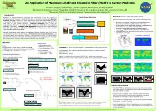
This article discusses the use of the Maximum Likelihood Ensemble Filter (MLEF) in addressing carbon problems. The MLEF calculates optimal estimates of model state variables, empirical parameters, model error, and boundary conditions error. It also calculates the uncertainty of these estimates and provides more information about the probability distribution function. The MLEF uses a fully non-linear approach and does not require adjoint models. It has been applied to various carbon studies such as parameter estimation, estimating uncertainties of carbon fluxes and empirical parameters, and utilizing various observations of weather and CO2. Preliminary results using the MLEF in hurricane simulations have shown promising improvements in analysis results.

E N D
Maximum Likelihood Ensemble Filter:application to carbon problems Prepared by Dusanka Zupanski and ……
Maximum Likelihood Ensemble Filter (MLEF)(Zupanski 2005; Zupanski and Zupanski 2005) • Developed using ideas from: • Variational data assimilation(3DVAR, 4DVAR) • Iterated Kalman Filters • Ensemble Transform Kalman Filter (ETKF, Bishop et al. 2001) Characteristics of the MLEF • Calculates optimal estimatesof: - model state variables (e.g., carbon fluxes, sources, sinks) - empirical parameters (e.g., light response, allocation, drought stress) - model error (bias) - boundary conditions error (lateral, top, bottom boundaries) • Calculates uncertainty of all estimates • Fully non-linear approach. Adjoint models are not needed. • Provides more information about PDF (higher order moments could be calculated from ensemble perturbations) • Non-derivative minimization (first variation instead of first derivative is used). Dusanka Zupanski, CIRA/CSU Zupanski@CIRA.colostate.edu
MLEF APPROACH Minimize cost function J Change of variable (preconditioning) - model state vector of dim Nstate >>Nens - control vector in ensemble space of dim Nens - information matrix of dim Nens Nens Dusanka Zupanski, CIRA/CSU Zupanski@CIRA.colostate.edu
MLEF APPROACH (continued) Analysis error covariance Forecast error covariance Forecast model M essential for propagating in time (updating) columns of Pf. Dusanka Zupanski, CIRA/CSU Zupanski@CIRA.colostate.edu
Ideal Hessian Preconditioning VARIATIONAL MLEF Milija Zupanski, CIRA/CSU ZupanskiM@CIRA.colostate.edu
STATE AUGMENTATION APPROACH as a part of the MLEF Example: parameter estimation - augmented state variable - augmented forecast model Parameters are randomly perturbed only in the first cycle. In later cycles, the MLEF updates ensemble perturbations. Assumption: parameter remains constant, or changes slowly with time SAME FRAMEWORK IS USED FOR MODEL BIAS ESTIMATION (use bias instead of a parameter to augment state variable)
Applications of the MLEF to carbon studies • TRANSCOM - …. -….(Ravi, perhaps you can include a couple of bullets for Transcom) • SiB Parameter estimation - Estimate control parameters on the fluxes - MLEF calculates uncertainties of all parameters (in terms of Pa and Pf) • LPDM - Estimate monthly mean carbon fluxes, empirical parameters - Estimate uncertainties of the mean fluxes and empirical parameters • SiB-CASA-RAMS - Use various observations of weather, eddy-covariance fluxes, CO2 - Estimate carbon fluxes, empirical parameters (e.g., light response, allocation, drought stress, phonological triggers) - Time evolution of state variables, provided by the coupled model, is critical for updating Pf Dusanka Zupanski, CIRA/CSU Zupanski@CIRA.colostate.edu
TRANSCOM Ravi, you might want to add more detail about TRANSCOM Dusanka Zupanski, CIRA/CSU Zupanski@CIRA.colostate.edu
Preliminary results using RAMS • Hurricane Lili case • 35 1-h DA cycles: 13UTC 1 Oct 2002 – 00 UTC 3 Oct • 30x20x21 grid points, 15 km grid distance (in the Gulf of Mexico) • Control variable: u,v,w,theta,Exner, r_total (dim=54000) • Model simulated observations with random noise (7200 obs per DA cycle) • Nens=50 • Iterative minimization of J (1 iteration only) RMS errors of the analysis (control experiment without assimilation) Hurricane entered the model domain. Impact of assimilation more pronounced. Dusanka Zupanski, CIRA/CSU Zupanski@CIRA.colostate.edu
Example: Total humidity mixing ratio, level=200 m, cycle 31 TRUTH NO ASSIMILATION ASSIMILATION Locations of min and max centers are much improved in the experiment with assimilation.
SUMMARY • The MLEF is currently being evaluated in various atmospheric science applications, showing encouraging results. • The MLEF is suitable for assimilation of numerous new carbon observations, employing complex non-linear coupled models. • Work in carbon applications has just started. Results will be presented in the future. Dusanka Zupanski, CIRA/CSU Zupanski@CIRA.colostate.edu