Download
1 / 42
430 likes | 845 Views
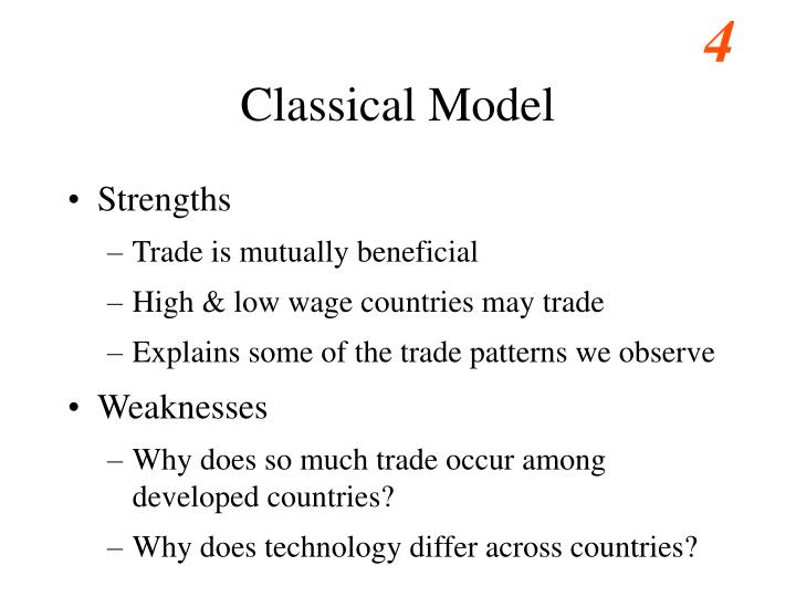
Classical Model. Strengths Trade is mutually beneficial High & low wage countries may trade Explains some of the trade patterns we observe Weaknesses Why does so much trade occur among developed countries? Why does technology differ across countries?. Heckscher-Ohlin (HO) Model.

E N D
Classical Model • Strengths • Trade is mutually beneficial • High & low wage countries may trade • Explains some of the trade patterns we observe • Weaknesses • Why does so much trade occur among developed countries? • Why does technology differ across countries?
Heckscher-Ohlin (HO) Model • Built upon observed differences among • Factors that countries possess • Factors required to produce various goods • Insights • Causes of trade • Effects of trade on factor prices • Effect of economic growth on trade patterns • Political behavior
Assumptions for HO Model • Keep assumptions 1 through 10 • Drop assumptions 11 & 12 • Add assumptions 13 through 17
Assumption #13 • There are two factors of production, labor (L), and capital (K). Owners of capital are paid a rental payment (R) for the services of their assets, and labor receives a wage payment (W).
Assumption #14 • The technologies available to each country are identical. • Any technology is available to any country • Factor prices determine the technology chosen
Unit Capital input aTS , in machines per bushel Input combinations that produce one bushel of Soybeans // Unit Labor input aLF , in hours per bushel A Model of a Two-Factor Economy Compare to Figure 4-1: Input Possibilities in Soybean Production
Assumption #15 • The production of T is labor intensive relative to the production of S • That is, T requires more labor per machine • Implies that production of S is capital intensive (relative to the production of T). • That is, S requires more machines per worker
K per Worker for US Industries Thousands of 1972 dollars. Item 4.1, page 89, 5th edition, Husted & Melvin
Wage-rental ratio, w/r 1 2 Capital-labor ratio, K/L Factor Prices and Input Choices Which line represents the Capital-intensive industry, 1 or 2? Compare to Figure 4.2, page 70
Wage-rental ratio, w/r TT SS Capital-labor ratio, K/L Factor Prices and Input Choices Soybean production is capital-intensive at any given wage/rental ratio
Wage-rental ratio, w/r TT SS (w/r)2 (w/r)1 PW Capital- labor Ratio, K/L Relative price of T, PT/PS (PT/PS)1 (PT/PS)2 (KT/LT)1 (KS/LS)1 (KT/LT)2 (KS/LS)2 Increasing Increasing Combing Figures 4-2 and 4-3 Compare to Figure 4-4, page 71
Assumption #16 • Country A is relatively capital abundant, while B is labor abundant.
K per Worker: Selected Countries 1985 international prices. Item 4.2, page 91, 5th edition Husted & Melvin
Quantity definition of factor abundance • Country A is relatively capital abundant, if the ratio of its capital stock to its labor force (K/L) is greater than that of the other country:
Price definition of factor abundance • Country A is relatively capital abundant, if its wage-rental ratio (W/R) is higher than the other country’s wage-rental ratio:
Strong factor abundance assumption • If country A is relatively capital abundant, by the quantity definition, its wage-rental ratio (W/R) will be higher than the other country’s wage-rental ratio. • That is, the price definition holds, too.
Increasing Opportunity Cost in A S is K-intensive A is K-abundant 20 18 14 America’s PPF TEXTILES, T (millions of yards per year) 12 6 0 2 4 8 12 10 16 SOYBEANS, S (millions of bushels per year)
Increasing Opportunity Cost in B T is L-intensive B is L-abundant 40 TEXTILES, T (millions of yards per year) 20 Britain’s PPF 0 5 10 SOYBEANS, S (millions of bushels per year)
Assumption #17 • Tastes in the two countries are identical. • Given same GDP & prices, same choice • Implies that supply conditions alone determine the direction of comparative advantage (CA). • Different tastes would imply different demand • Could reverse the direction of CA.
Rybczynski Theorem • At constant world prices, if a country experiences an increase in the supply of one factor, it will produce more of the product intensive in that factor and less of the other. • See Figure 4.5 , page 73, and 4.6, page 74 Krugman & Obstfeld
L__ O_ __ 1 K_ K_ __ O_ L_ Increasing Increasing Increasing Increasing Which is the K-intensive industry? Labor used in _____________ production Capital used in ________ production Capital used in _____ production Labor used in______production Compare to Figure 4-5, page 73
LS OS T 1 KT KS S OT LT Increasing Increasing Increasing Increasing S is K intensive, T is L intensive Labor used in Soybean production Capital used in Textile production Capital used in S production Labor used in Textile production
Rybczynski Theorem • How do the outputs of the two goods change when the economy’s resources change? • Increase the amount of one factor, say K, and observe the results
O2S L1S L2S O1S K1T 1 K1S T K2T K2S 2 S1 S2 OT L1T L2T Increasing Increasing Increasing Increasing K increases. S (K int.) expands. S needs more labor. T must contract L used in S production K used in S production K used in T production L used in T production
Output of T, QT Slope = -PS/PT Slope = -PS/PT Output of S, QS An increase in K in Country A. 1 Q1T 2 Q2T PPF2 PPF1 Q1S Q2S
Output of T, QT 2 Slope = -PS/PT Q2T Slope = -PS/PT Q1T 1 PPF2 PPF1 Output of S, QS Q2S Q1S An increase in L in country B. Compare to Figure 4-7, page 75. Now try it yourself – solve problem 2
Rybczynski Theorem • Also helps us to understand that an economy will tend to be more productive in industries that use its abundant factor intensively.
Heckscher-Ohlin Theorem • A country will export the goods whose production is intensive in the factor with which that country is abundantly endowed.
Autarky in A 18 a 15 CIC0 TEXTILES, T (millions of yards per year) 12 0 13 10 16 SOYBEANS, S (millions of bushels per year)
Autarky in B 40 a 30 CIC0 TEXTILES, T (millions of yards per year) 20 Britain’s PPF 10 0 4 6.5 9 SOYBEANS, S (millions of bushels per year)
Relative price of S, ______ RSB RSA 3 2 1 RD Relative quality of S, Trade Leads to a Convergence of Relative Prices Compare to Figure 4-8, page 77.
Relative price of S, PS/PT 3 1 Relative quality of S, QS + Q*S QT + Q*T Trade Leads to a Convergence of Relative Prices RSB RSA 2 RD
With free trade, there will be one world relative price for S (PS/PT) and T (PT/PS). • As PS/PT rises in Country A, their S industry expands while their T industry contracts. • As PS/PT falls in Country B, their S industry contracts while their T industry expands. • Tricky to draw the general equilibrium solution, so let’s try it together.
International Trade Equilibrium • Incomplete specialization in Comparative Advantage good. • Community Indifference Curve (CIC) & Terms of Trade line (ToT) tangent at consumption point • Congruent trade triangles imply balanced trade.
Stolper-Samuelson Theorem • Free international trade benefits the abundant factor and harms the scarce factor.
As PS/PT rises in Country A, PT/PS and w/r fall. • Look back at Figure 4-4, or slide 15. • A is K abundant (L scarce) • As PS/PT falls in Country B, PT/PS and w/r rise. • B is L abundant (K scarce)
Factor-Price Equalization (FPE) Theorem • Given all the assumptions of the HO model, free trade will lead to the international equalization of individual factor prices. • Look again at Figure 4-4, or slide 15. • One relative price for T, PT/PS • One wage-rental ratio, w/r
Factor-Price Equalization? “There isn’t any.” Why not? • Some goods are not produced in some countries. • Productivity (technology) does differ between countries. • Goods’ prices differ due to natural and artificial barriers to trade.
Learning Objectives • Examine the need to build a new model • Understand five more assumptions • Prove HO Theorem • Prove Rybczynski Theorem • Prove Factor-Price Equalization Theorem • Prove Stolper-Samuelson Theorem • Introduce Specific-Factors Model
Specific-Factors Model • Keep all HO assumptions except: • one factor is immobile (say K) • different rental rates for machines in S & T industries • Labor still mobile, implying one wage, W • W = VMPS = PS x MPLS • Appendix 4.2, pages 118-120, Husted & Melvin. See Figures A4.5 and A4.6
Specific-Factors Model • W = VMPS = PS x MPLS • W = VMPT = PT x MPLT