Nanostructures and Quantum Effects in Nanodevices

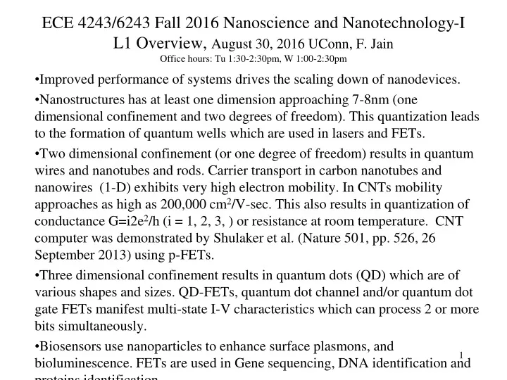
1. ECE 4243/6243 Fall 2016 Nanoscience and Nanotechnology-I L1 Overview, August 30, 2016 UConn, F. Jain Office hours: Tu 1:30-2:30pm, W 1:00-2:30pm Improved performance of systems drives the scaling down of nanodevices. Nanostructures has at least one dimension approaching 7-8nm (one dimensional confinement and two degrees of freedom). This quantization leads to the formation of quantum wells which are used in lasers and FETs. Two dimensional confinement (or one degree of freedom) results in quantum wires and nanotubes and rods. Carrier transport in carbon nanotubes and nanowires (1-D) exhibits very high electron mobility. In CNTs mobility approaches as high as 200,000 cm2/V-sec. This also results in quantization of conductance G=i2e2/h (i = 1, 2, 3, ) or resistance at room temperature. CNT computer was demonstrated by Shulaker et al. (Nature 501, pp. 526, 26 September 2013) using p-FETs. Three dimensional confinement results in quantum dots (QD) which are of various shapes and sizes. QD-FETs, quantum dot channel and/or quantum dot gate FETs manifest multi-state I-V characteristics which can process 2 or more bits simultaneously. Biosensors use nanoparticles to enhance surface plasmons, and bioluminescence. FETs are used in Gene sequencing, DNA identification and proteins identification.

2. Overview Does scaling down to sub-7nm feature size (e.g. FETs or quantum dot lasers) leads to novel phenomena that provide new device characteristics due to quantum effects? Photonic devices, MEMs, and biosensors miniaturization leads to nanostructures. Si Nanophotonics provides a way to integrate electronic and photonic devices on same substrate. 4. Electronic and photonic devices involve p-n homo- and heterojunctions, FETs and memory devices. P-n junctions are basic to LEDs, lasers, photodetectors, MOS imaging and displays, and solar cells. 5. Carrier transport and optical transitions in 1-D (e.g. carbon nanotubes and nanowires), 2-D (e.g. graphene, MoSe2, quantum well layers), and 0-D quantum dot based layers requires carrier concentration (density of states and Fermi-Dirac statistics, phonons) and tunneling through barriers. 6. Fabrication of nanostructures is dependent on materials processing.

3. Overview cont. 1. Quantum effects manifests when at least one dimension where electrons exist become comparable to 5-8nm. 2. One-dimensional constraint results in the formation of quantum wells, multiple quantum wells, and superlattices. Energy density of states in quantum wells is different than in layers which are not constrained (called 3-d or bulk material). Two-dimensional graphene does not exhibit a band gap until an electric field is applied. Field-induced band gap has been observed. 3. Two-dimensional constraints result in the formation of nanowires, nanotubes. Energy density of states in quantum wires/nanotubes is different than in quantum wells. 4. The effective band gap in quantum wells is higher than bulk layer and band gap in nanowire/tube is higher than in a well. 5. Photon absorption or emission involves electronic transitions which depend on the density of states. Absorption coefficient in quantum wires is higher than in wells. It also starts at higher energy than band gap in bulk materials.

4. Overview cont. 6. Quantum wells are realized using barrier layers (e.g. AlGaAs barrier and GaAs well). Their shapes may be rectangular, parabolic, or mixed. Energy levels are obtained by solving Schrodinger equation using appropriate boundary conditions shape and effective mass of the material. 7. Carriers may tunnel from one quantum well to other or one quantum well to quantum dot if they are in vicinity and a finite probability exist. The probability or rate of tunneling is computed by solving the Schrodinger equation in various regions and finding the relative amplitude of wavefunctions. 8. Optical transitions may involve free carriers or formation of excitons. 9. Most of the electronic and photonic devices use semiconductor materials. 10. Semiconductors are direct energy gap or indirect gap. Metals do have not energy gaps. Insulators have above 4.0eV energy gap.

5. Examples of Nanodevices (p. 5) A. Hokazono, k. Ohuchi, M. Takayanagi, Y. Watanabe, S. Magoshi, Y. Kato, T. Shimizu, S. Mori, H. Oguma, T. Sasaki, H. Yoshimura, K. Miyano, N. Yasutake, H. Suto, K. Adachi, H. Fukui, T. Watanabe, N. Tamaoki, Y. Toyoshima, and h. Ishiuchi, “14 nm gate length CMOSFETs utilizing low thermal budget process with poly SiGe and Ni salicide,” IEDM Tech. Digest, p. 639, December 2002. Fig. 7. Topology of a 14 nm fabricated FET. Fig. 1. A typical MOSFET with sub-30nm channel. Fig. 5. Topology of a fabricated FINFET. Ref. Bin Yu, L. Chang, S. Ahmed, H. Wang, S. Bell, C. Yang, C. Tabery, C. Ho, Q. Xiang, T-J. King, J. Bokor, C. Hu, M-R. Lin, and D. Kyser, “FinFET Scaling to 10nm Gate Length,” IEDM Tech. Digest, p. 251, December 2002. Fig .2. Schematic cross-section of a floating Fig .4 energy band model to program a

6. Examples of Quantum dot lasers (p.8-9)

7. Why quantum well, wire and dot lasers, modulators and solar cells? Quantum Dot Lasers: • Low threshold current density and improved modulation rate. • Temperature insensitive threshold current density in quantum dot lasers. Quantum Dot Modulators: • High field dependent Absorption coefficient (α ~160,000 cm-1) : Ultra-compact intensity modulator • Large electric field-dependent index of refraction change (Δn/n~ 0.1-0.2): Phase or Mach-Zhender Modulators Radiative lifetime τr ~ 14.5 fs (a significant reduction from 100-200fs). Quantum Dot Solar Cells: High absorption coefficent enables very thin films as absorbers. Excitonic effects require use of pseudomorphic cladded nanocrystals (quantum dots ZnCdSe-ZnMgSSe, InGaN-AlGaN) Table I Computed threshold current density (Jth) as a function of dot size infor InGaN/AlGaN Quantum Dot Lasers (p.11) (Ref. F. Jan and W. Huang, J. Appl. Phys. 85, pp. 2706-2712, March 1999).

8. Quantum confinement of carriers • Energy bands and carrier concentrations. • Density of states in bulk, quatnum wells, quantum wires/nanotubes, nano-rods and quantum dots. • Confinement and tunneling of carriers across potential barriers.

9. Optical transitions in nanostructures • Band to band free carrier transitions. • Band to band transitions involving exciton formation. • Light emission and absorption.

10. Energy bands Fig. 8 and 9. p.119

11. V(R) V0 2b<a -b 0 a a+b Energy bands (Ref. F. Wang, “Introduction to Solid State Electronics”, Elsevier, North-Holland) Fig. 13(b) and Fig. 13c. p.123-124

12. Absorption and emission of photons 1) (Transition Probability) here, (h) is the joint density of states in a volume V (the number of energy levels separated by an energy Fig. 2 p.138 2) Pmo probability that a transition has occurred from an initial state ‘0’ to a final state ‘m’ after a radiation of intensity I(h) is ON for the duration t. The joint density of states is expressed as Eq. 2B) o

13. Time dependent Schrodinger Equation p.68-69

15. Infinite Potential Well p.47 Solve Schrodinger Equation In a region where V(x) = 0, using boundary condition that (x=0)=0, (x=L)=0. Plot the (x) in the 0-L region.

16. In the region x = 0 to x = L, V(x) = 0 Let (2) The solution depends on boundary conditions. Equation 2 can be written as D coskxx + C sinkxx. At x=0, (3) , so D= 0 nx = 1,2,3… (4) Using the boundary condition (x=L) = 0, we get from Eq. 3 sin kxL = 0, L = Lx

17. Page 52-53: Using periodic boundary condition (x+L) = (x), we get a different solution: We need to have kx= ---(6) The solution depends on boundary conditions. It satisfies boundary condition when Eq.6 is satisfied. If we write a three-dimensional potential well, the problem is not that much different ky = n y= 1,2,3,… kZ = , n z = 1,2,3,…. …(7) The allowed kx, ky, kz values form a grid. The cell size for each allowed state in k-space is …(8)

18. E N(E) VB k k+dk Density of States in 3D semiconductor film (pages 53, 54) Density of states between k and k+dk including spin N(k)dk = …(10) …11 Density of states between E and E+dE N(E)dE=2 E=Ec + (12) …(13) N(E)dE = …14 N(E)dE = …15

19. AlxGa1-xAs AlxGa1-xAs GaAs V(z) ∆EC ∆Ec = 0.6∆Eg ∆Ev = 0.4∆Eg 0 z 0 ∆EV -EG z ∆EV -EG+∆EV Finite Potential Well p.70

20. In the barrier region

21. Wavefunction matching at well-barrier boundary

22. Wavefunction matching at well-barrier boundary

25. kL/2 αL/2 Where, radius is Output: Equation (15) and (12), give k, α’ (or α). Once k is known, using Equation (4) we get: The effective width, Leff can be found by: E1 is the first energy level. (4)

26. AlxGa1-xAs AlxGa1-xAs GaAs V(z) ∆EC ∆Ec = 0.6∆Eg ∆Ev = 0.4∆Eg 0 z 0 ∆EV -EG z ∆EV -EG+∆EV Summary of Schrodinger Equation in finite quantum well region. (1) In the well region where V(x) = 0, and in the barrier region V(x) = Vo = ∆Ec in conduction band, and ∆Ev in the valence band. The boundary conditions are: (5) Continuity of the wavefunction (6) Continuity of the slope Eigenvalue equation:

27. C. 2D density of state (quantum wells) page 84 Carrier density number of states (1) Without f(E) we get density of states Quantization due to carrier confinement along the z-axis.

28. Density of states summary

29. Nanophotonics • Si nanophotonics • Surface enhanced Raman effect via plasmon formation in thin metal films or gold nanoparticles. • Plasmons are modified by functionalized nanoparticles enabling biosensing of proteins etc.

30. Figure 1: Simple examples of 1D, 2D, and 3D photonic crystals. The different colors represent materials with different refractive indexes. Ref: Photonc Crystals: Molding the Flow of Light, by J. D. Joannopoulos Si Nanophotonics(pp. 60-65) Photons are confined in a waveguide which comprise of a higher index of refraction layer (waveguide) sandwiched between two lower index (or cladding) layers). If there is a stack of these layers and spacing between cladding and waveguide layer is such that there is coupling between waveguides, we have a 1D photonic crystal which allows certain wavelengths and blocks others. This is considered having a photonic band gap. If this is done in two dimensions, we have a 2D photonic crystal as shown below. 2D and 3D photonic crystals are used to design narrow waveguides which can turn light 90 degrees. A physical device that possesses a photonic band gap (PBG) can be classified as a PBG structure. A photonic band gap is similar to the band gap of a semiconductor material, except that instead of comprising a range of energies, a PBG consists of a range of optical frequencies that cannot exist in the structure. PBGs arise because of the symmetry of a structure. For example, for a DBR (refer to previous write up on DBRs), a basic type of PGB structure, the PBG exists only for light normal to the plane of incidence. If the wavelength of light incident on the DBR is close enough to the wavelength for which it was designed, the light will be reflected at each layer interface. The light penetrating into the DBR is evanescent, i.e. decaying exponentially. Thus, modes within a frequency range centered at a frequency corresponding to this wavelength cannot exist within the DBR. We designate this range of frequencies the PBG of this particular DBR structure (it is possible for a structure to have multiple PBGs).

31. Nanophotonics (pp.506-508)

32. Biophotonics Figs. 6(a) and 6(b) address DNA/gene sequencing describing current methods (using optical detection and pyro-sequencing) and the emerging methods (chem-FET based pH sensing21). Figure 6(a) shows a system view with details in Figs. 6(b) and additional details in Fig. 12. The new electronic method provides faster DNA synthesis/gene sequencing22-23 in contrast to luminescence-based pyro-sequencing methods24. A one-hour teaching module (Figure 6) will expose students how a transistor (FET) can sense the H+ concentration (or pH value), which depends on number of bases of a reference DNA matching with the bases of a gene fragment DNA present in a target solution. Figs. 7(a) and 7(b) show how an implantable sensor monitors glucose levels by producing a current.

33. Semiconductor Background Review Energy bands in semiconductors: Direct and indirect energy gap N- and p-type doping, Carrier concentrations: n*p=ni2 Fermi-Dirac Statistics & Fermi level Drift and diffusion currents P-n junctions: Forward/Reverse biased Heterojunctions

34. UCONN ECE 4243/6243 Fall 2014 Nanoscience and Nanotechnology-I L2 Energy levels in potential wells and density of states Bonds and energy bands (page 38)

35. Bonds (page 43) Tetrahedral primitive cell of Si lattice Fig. 15. Schematic representation of s, py, sp3, and tetrahedral orbitals

36. Conductivity σ, Resistivity ρ= 1/σ Current density J in terms of conductivity s and electric field E: J = s E = s (-V) = - sV I = J A = s E (W d), In n-type Si, sn= q mn nno + q mp pno

37. Carrier Transport: Drift and Diffusion Drift Current: In = Jn A = - (q mn n) E A Diffusion Current density: Jn= +q Dnn, [Fick's Law] Total current = Diffusion Current + Drift Current Einstein’s Relationship: Dn/μn =kT/q Pnonno=ni2 n-Si ND=Nn=nno Pponpo=ni2 p-Si NA=Pp=Ppo

38. Drift and Diffusion of holes in p-Si In p-type Si, The conductivity is: sn= q mp ppo + q mn npo Drift Current: Ip drift = Jp A = (q mp p) E A Diffusion Current density: Jp= - q Dpp, [Fick's Law] Diffusion current: Ip diff = - q A Dpp Einstein’s Relationship: Dn/μn =kT/q Total hole current = Diffusion Current + Drift Current Ip= - q A Dpp + (q mp p) E A

39. Carrier concentration When a semiconductor is pure and without impurities and defects, the carrier concentration is called intrinsic concentration and it is denoted by ni. i.e. n=p=ni. ni as a function of Temperature, see Figure 17 (page 28) and Fig. 11 (page 69). Also, ni can be obtained by multiplying n and p expressions (apge 68 of notes)

40. Extrinsic Semiconductors: Doped n- and p-type Si, GaAs, InGaAs, ZnMgSSe IIIrd or Vth group elements in Si and Ge are used to dope them to increase their hole and electron concentrations, respectively. Vth group elements, such as Phosphorus, Arsenic, and Antimony, have one more electron in their outer shell, as a result when we replace one of the Si atoms by any one of the donor, we introduce an extra electron in Si. These Vth group atoms are called as donors. Once a donor has given an electron to the Si semiconductor, it becomes positively charged and remains so. Whether a donor atom will donate its electron depends on its ionization energy ED. If there are ND donor atoms per unit cm3, the number of the ionized donors per unit volume is given by

41. Fermi-Dirac Statistics We have used a statistical distribution function, which tells the probability of finding an electron at a certain level E. This statistics is called Fermi-Dirac statistics, and it expresses the probability of finding an electron at E as Ef is the energy at which the probability of finding an electron is ½ or 50%. In brief, donor doped semiconductors have more electrons than holes. E

42. Acceptors and p-type semiconductors: We can add IIIrd group elements such as Boron, Indium and Gallium in Si. When they replace a Si atom, they cause a deficiency of electron, as they have three electrons in their outer shell (as compared to 4 for Si atom). These are called acceptor atoms as they accept electrons from the Si lattice which have energy near the valence band edge Ev. Eq. 12 expresses the concentration of ionized acceptor atoms (on page 71). N-A is the concentration of the ionized acceptor atoms that have accepted electrons. EA is the empty energy level in the acceptor atom. Hole conduction in the valence band: The electron, which has been accepted by an acceptor atom, is taken out of the Si lattice, and it leaves an empty energy state behind. This energy state in turn is made available to other electrons. It is occupied by other electrons like an empty seat in the game of musical chairs. This constitutes hole conduction.

43. Donors and acceptors in compound semiconductors (see Problem set before chapter 1, p. 26)Semiconductors such as GaAs and InGaAs or ZnMgSSe are binary, ternary, and quaternary, respectively. They represent III-V and II-VI group elements. For example, the doping of GaAs needs addition of group II or VI elements if we replace Ga and As for p and n-type doping. In addition, we can replace Ga by Si for n-type doping. Similarly, if As is replaced by Si, it will result in p-type doping. So Si can act as both n and p-type dopant depending which atom it replaces. Whether Si is donor or acceptor depends on doping temperature.

44. Calculation of electron and hole concentrations in n-type and p-type semiconductors Method #1: (simplest) Simple expressions for electron and hole concentrations in n-Si having ND concentration of donors (all ionized). Electron concentration is n = nn or nno =ND, (here, the subscript n means on the n-side or in n-Si; additional subscript ‘o’ refers to equilibrium). Hole concentration is pno =ni2/ND. For p-Si having NA acceptor concentration (all ionized), we have p= pp =NA, and electron concentration npo= (ni2)/NA, Method#2 (simpler) Here, we start with the charge neutrality condition. Applying charge neutrality, we get: total negative charge density = total positive charge density i.e. qND+ + qpno = qnno, here pno and nno are the hole concentrations in the n-type Si at equilibrium. But pno or hole concentration = ni2/ND.Substituting pno in the charge neutrality equation, we get electron concentration by solving a quadratic equation [Eq 8, page 71]. Its solution is:

45. Method#3 (Precise but requires Ef calculations) qND+ + qpno = qnno, Charge neutrality condition in n-type semiconductor can be written as:[Eq. 6 on page 70] Here, we have ignored the factor of ½ from the denominator of the first term. In this equation, we know all parameters except Ef. One can write a short program and evaluate Ef or assume values of Ef and see which values makes left hand side equal to the right hand side.

46. Effect of Temperature on Carrier Concentration The intrinsic and extrinsic concentrations depend on the temperature. For example, in Si the intrinsic concentrations at room temperature (~300K) is ni =1.5x1010 cm-3. If you raise the temperature, its value increases exponentially (see relation for ni).

47. Carrier concentration expression [review pages 53-59] The electron concentration in conduction band between E and E+dE energy states is given by dn = f(E) N(E) dE. To find all the electrons occupying the conduction band, we need to integrate the dn expression from the bottom of the conduction band to the highest lying level or energy width of the conduction band. That is, [see page 56 notes] The density of states N(E) will change if we are dealing with quantum wells, wires, dots. This leads to electron concentration (see page 57): This equation assumes that the bottom of the conduction band Ec = 0. An alternate expression results, if Ec is not assumed to be zero.

48. ·Direct and Indirect Energy Gap Semiconductors Fig. 10b. Energy-wavevector (E-k) diagrams for indirect and direct semiconductors (page 17). Here, wavevector k represents momentum of the particle (electron in the conduction band and holes in the valence band). Actually momentum is = (h/2p)k = k

49. Electrons & Holes Photons Phonons Statistics F-D & M-B Bose-Einstein Bose-Einstein Velocity vth ,vn 1/2 mvth2 =3/2 kT Light c or v = c/nr nr= index of refraction Sound vs = 2,865 meters/s in GaAs Effective Mass mn , mp (material dependent) No mass No mass Energy E-k diagram Eelec=25meV to 1.5eV ω-k diagram (E=hω) ω~1015 /s at E~1eV Ephotons = 1-3eV ω-k diagram (E= ω) ω~5x1013/s at E~30meV Ephonons = 20-200 meV Momentum P= k k=2π/λ λ=2πvelec/ω momentum: 1000 times smaller than phonons and electrons P= k k=2π/λ λ=2πvs/ω (page 17).

50. P-n Junctions (pp. 20-28) Use (Vbi – Vf) for forward-biased junctions, and (Vbi + Vr ) for reverse-biased junctions.