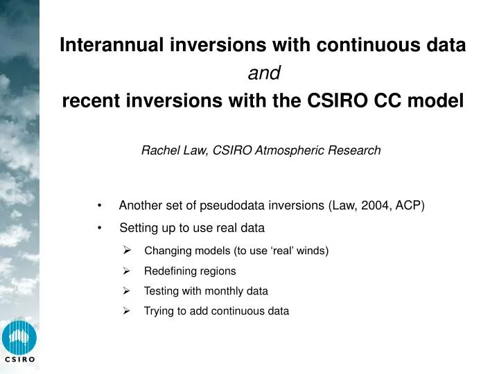
Interannual inversions with continuous data and recent inversions with the CSIRO CC model

1. Interannual inversions with continuous data and recent inversions with the CSIRO CC model Rachel Law, CSIRO Atmospheric Research • Another set of pseudodata inversions (Law, 2004, ACP) • Setting up to use real data • Changing models (to use ‘real’ winds) • Redefining regions • Testing with monthly data • Trying to add continuous data

2. Continuous data at Cape Grim (purple) and Aspendale (blue) Wind speed > 2.5 m/s

3. AIM: Perform a T3L3 type inversion using pseudodata generated from interannually-varying fluxes (Friedlingstein land, LeQuere ocean) and compare results using monthly and 4 hourly data at 35 sites for 1982-1997 BUT problem of size T3-IAV base case (78 sites, solve 86-02): nsrc=4557, ndat=14040 116 region inversion, 35 sites with 4hr data, if solved over 86-02: nsrc=23665, ndat=1149750 SOLUTION: Solve in 2 year overlapping segments adding 1 new year of data each time. Predicted sources from previous step used as priors in next step. SHORT-CUT: Full covariance matrix not kept from one step to the next (but tests showed this wasn’t a problem)

4. Two example regions Comparison with correct sources (black) and between 3 year inversion (red) and 1 year inversions (green, blue)

5. Difference in 1982-1997 mean source from correct source in gCm-2yr-1 (yellow/green good, blue/red bad) Using 4 hr data Some large biases over land regions – no significant improvement over monthly data Using monthly data

6. Root mean square bias in the mean seasonal cycle in gCm-2yr-1 (blue good, red bad) Using 4 hr data Regions with sites nearby generally better than with monthly data Using monthly data

7. Correlation of interannual variability between estimated and correct(red good, blue bad) Using 4 hr data Higher correlations over more regions (53 > 0.6) than with monthly data (17 > 0.6). Some low correlations over ocean – leakage of land signal. Using monthly data

8. Magnitude of interannual variability compared to correct(red variability too large, blue variability too small) Using 4 hr data Variability too small or too large away from sites Using monthly data Magnitude of variability underestimated for land regions away from sites

9. CSIRO Conformal-Cubic Atmospheric Model (CCAM) Stand-alone GCM or nudged with NCEP winds. Uniform or stretched grid. Currently using ~200 km. Trace gas transport using prescribed sources and on-line biospheric CO2. Inversion set-up: 94 land regions, (42 also day-time flux), 46 (48) ocean regions. 6 month responses (hourly resolution) currently run for 1995, 1996, 1997.

10. Inversion using 1992-2002 monthly data only – 88 sites (81 GV, 7 WDCGG), data uncertainty: 1.5*rsd Prior source: Fos95+CASA NEP+Taka (but no presub fields used) Prior source uncertainty: ocean, area*150 gCm-2yr-1 land, tree area*1500+grass area*800+desert area*100 gCm-2yr-1 Total land – green Total ocean – blue Solid CCAM, dashed TC mean

11. Australian region source (12 month running mean) compared to TransCom mean Note: CCAM case is sum of 16 regions, TransCom is one region and includes New Zealand. TC sources are sensitive to Baring Head CCAM NZ source

12. Standard deviation of interannual component of fluxes in gCm-2yr-1 Prior source uncertainty in gCm-2yr-1

13. Adding continuous data A small first step: use estimated sources and uncertainties from inversion with monthly data as prior sources for this inversion. Run inversion for 1 site (Cape Grim, 1997 hourly data). What data uncertainty is appropriate? Blue – obs green – unc 1.4 ppm red – unc 28 ppm

14. Change in 1997 mean source and uncertainty estimates with data uncertainty for four example regions Blue – SE coast, mainland Australia Red – ocean to SW of Cape Grim Blue – Western Brazil Red – Western Siberia

15. Ratio of estimated to prior uncertainty (for 1997 mean source) due to addition of Cape Grim hourly data with 7 ppm data uncertainty

16. Tasmania source estimate Blue – original prior source, red – source from inversion of monthly data, green – set of inversions using hourly CGA with different data uncertainty, pale blue – smallest data uncertainty (1.4 ppm) Source uncertainty shown by dashed line, mid-range (14ppm) case shown for set of inversions Monthly data added little information about Tasmanian source, CGA data tends to weaken seasonal cycle. Note some months much better observed (e.g. Feb) than others (e.g. May). Larger shifts from prior in better observed months.

17. SE Australia source estimate Blue – prior, red – monthly inversion, green - CGA hourly data Monthly data moves sources closer to zero, reduces spring uptake, but only small reduction in uncertainty Hourly data reduces seasonality further, tendency to shift uptake from Nov to Sep-Oct. Substantial decrease in uncertainty.

18. Ocean to south west of Cape Grim Blue – prior, red – monthly inversion, green – hourly CGA data Monthly data put large seasonality into region compared to Takahashi prior Hourly data tends to moderate seasonality and make more consistent with Takahashi

19. Australian continental source Red – monthly inversion, blue – addition of hourly Cape Grim Thick dashed line – 12 month running mean Lose spring uptake and consequently shift annual mean. Result seems unlikely.

20. Future plans • ‘Clean up’ method where possible e.g. monthly and continuous data in same step • Use full covariance matrix in 2nd step • Add more continuous sites • Extend number of years • Think about how to assess results – how do we know what’s a good result? • Test temporal averaging of data • Are there any ways to deal with transport model error?

21. Future plans – part 2