Binary Image Analysis: Part 1 Readings: Chapter 3: 3.1, 3.4, 3.8

1. Binary Image Analysis: Part 1Readings: Chapter 3: 3.1, 3.4, 3.8 thresholding grayscale images connected components labeling

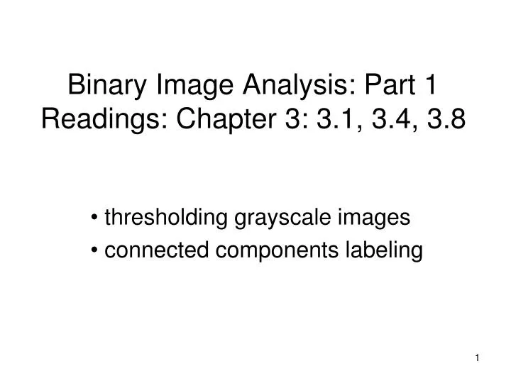
2. Binary Image Analysis Binary image analysis • consists of a set of image analysis operations • that are used to produce or process binary • images, usually images of 0’s and 1’s. • 0 represents the background • 1 represents the foreground 00010010001000 00011110001000 00010010001000

3. Binary Image Analysis • is used in a number of practical applications, e.g. • part inspection • riveting • fish counting • document processing

4. What kinds of operations? • Separate objects from background and from one another • Aggregate pixels for each object • Compute features for each object

5. Example: red blood cell image • Many blood cells are separate objects • Many touch – bad! • Salt and pepper noise from thresholding • How useable is this data?

6. Results of analysis • 63 separate objects detected • Single cells have area about 50 • Noise spots • Gobs of cells

7. Useful Operations • 1. Thresholding a gray-tone image • 2. Determining good thresholds • 3. Connected components analysis • 4. Binary mathematical morphology • 5. All sorts of feature extractors • (area, centroid, circularity, …)

8. Thresholding • Background is black • Healthy cherry is bright • Bruise is medium dark • Histogram shows two cherry regions (black background has been removed) This is abstract. How are histograms represented as data structures? pixel counts 0 256 gray-tone values

9. Histogram-Directed Thresholding How can we use a histogram to separate an image into 2 (or several) different regions? Is there a single clear threshold? 2? 3?

10. Automatic Thresholding: Otsu’s Method Grp 1 Grp 2 Assumption: the histogram is bimodal t Method: find the threshold t that minimizes the weighted sum of within-group variances for the two groups that result from separating the gray tones at value t. What is variance?

11. Computing Within-Group Variance • For each possible threshold t • For each group i (1 and 2) • compute the variance of its gray tones i2(t) • compute its weight qi(t) =  P() • where P() is the normalized histogram value for • gray tone , normalized by sum of all gray tones • in the image and called the probability of . • Within-group variance = q1(t) i2(t) + q2(t) i2(t) Grp 1 Grp 2 • in Grp i 0 255 t See text (Section 3.8) for the efficient recurrence relations; in practice, this operator works very well for true bimodal distributions and not too badly for others, but not the CTs.

12. Thresholding Example original gray tone image binary thresholded image

13. Connected Components Labeling Once you have a binary image, you can identify and then analyze each connected set of pixels. The connected components operation takes in a binary image and produces a labeled image in which each pixel has the integer label of either the background (0) or a component. connected components (shown in pseudo-color) binary image (after morphology)

14. Methods for CC Analysis • Recursive Tracking (almost never used) • Parallel Growing (needs parallel hardware) • Row-by-Row (most common) • Classical Algorithm (see text) • Efficient Run-Length Algorithm • (developed for speed in real • industrial applications)

15. Equivalent Labels Original Binary Image 0 0 0 1 1 1 0 0 0 0 1 1 1 1 0 0 0 0 1 0 0 0 1 1 1 1 0 0 0 1 1 1 1 0 0 0 1 1 0 0 0 1 1 1 1 1 0 0 1 1 1 1 0 0 1 1 1 0 0 0 1 1 1 1 1 1 0 1 1 1 1 0 0 1 1 1 0 0 0 1 1 1 1 1 1 1 1 1 1 1 0 0 1 1 1 0 0 0 1 1 1 1 1 1 1 1 1 1 1 0 0 1 1 1 0 0 0 1 1 1 1 1 1 1 1 1 1 1 1 1 1 1 1 0 0 0 1 1 1 1 1 1 1 1 1 1 1 1 1 1 1 1 0 0 0 1 1 1 1 1 1 0 0 0 0 0 1 1 1 1 1

16. Equivalent Labels The Labeling Process: Left to Right, Top to Bottom 0 0 0 1 1 1 0 0 0 0 2 2 2 2 0 0 0 0 3 0 0 0 1 1 1 1 0 0 0 2 2 2 2 0 0 0 3 3 0 0 0 1 1 1 1 1 0 0 2 2 2 2 0 0 3 3 3 0 0 0 1 1 1 1 1 1 0 2 2 2 2 0 0 3 3 3 0 0 0 1 1 1 1 1 1 11 1 1 1 0 0 3 3 3 0 0 0 1 1 1 1 1 1 1 1 1 1 1 0 0 3 3 3 0 0 0 1 1 1 1 1 1 1 1 1 1 1 1 1 1 1 1 0 0 0 1 1 1 1 1 1 1 1 1 1 1 1 1 1 1 1 0 0 0 1 1 1 1 1 1 0 0 0 0 0 1 1 1 1 1 1  2 1  3 What CSE algorithm does this kind of thing on a different structure?

17. Run-Length Data Structureused for speed of processing and to gain from hardware 0 1 2 3 4 0 1 2 3 4 1 1 1 1 1 1 1 1 1 1 1 1 1 1 1 row scol ecol label Binary Image 0 1 2 3 4 5 6 7 U N U S E D 0 0 0 1 0 0 3 4 0 1 0 1 0 1 4 4 0 2 0 2 0 2 4 4 0 4 1 4 0 Rstart Rend 0 1 2 3 4 • 2 • 4 • 6 • 0 0 • 7 7 Row Index Runs

18. Run-Length Algorithm Procedure run_length_classical { initialize Run-Length and Union-Find data structures count <- 0 /* Pass 1 (by rows) */ for each current row and its previous row { move pointer P along the runs of current row move pointer Q along the runs of previous row

19. Case 1: No Overlap Q Q |/////| |/////| |////| |///| |///| |/////| P P /* new label */ count <- count + 1 label(P) <- count P <- P + 1 /* check Q’s next run */ Q <- Q + 1

20. Case 2: Overlap Subcase 2: P’s run has a label that is different from Q’s run Subcase 1: P’s run has no label yet Q Q |///////| |/////| |/////////////| |///////| |/////| |/////////////| P P label(P) <- label(Q) move pointer(s) union(label(P),label(Q)) move pointer(s) }

21. Pass 2 (by runs) /* Relabel each run with the name of the equivalence class of its label */ For each run M { label(M) <- find(label(M)) } } where union and find refer to the operations of the Union-Find data structure, which keeps track of sets of equivalent labels.

22. Labeling shown as Pseudo-Color connected components of 1’s from thresholded image connected components of cluster labels