Download
1 / 24
240 likes | 417 Views
Ocean Syntheses. David Behringer NOAA/NCEP. NOAA Ocean Climate Observation 8th Annual PI Meeting June 25-27, 2012 Silver Spring, Maryland. Introduction. Ocean syntheses are constructed for many different purposes:

E N D
Ocean Syntheses David Behringer NOAA/NCEP NOAA Ocean Climate Observation 8th Annual PI Meeting June 25-27, 2012 Silver Spring, Maryland
Introduction • Ocean syntheses are constructed for many different purposes: • Regional analyses, high resolution now-casts, climate monitoring, initialization of seasonal or decadal forecasts, etc. • They employ a diversity of methods: • OI, 3D and 4D variational, adjoint, Kalman filtering and Kalman smoothing • They have a common requirement for observations: • Temperature and salinity profiles (BTs, CTDs, fixed moorings, Argo), altimetry, SST, SSS, etc. Here the focus will be on climate scale analyses and their ability to capture climate signals and how that is related to the availability of observations.
Comparison of Upper Ocean (0-300m) Heat Content (HC300) in Operational Analyses Xue et al., J. Clim., 2012
Comparison of HC300 in Operational Analyses Anomaly correlations of each analysis with EN3 for 1985-2009 Xue et al., J. Clim., 2012
Comparison of HC300 in Operational Analyses Ensemble Mean Linear Trend 1993-2009 Trend Normalized by Ensemble Spread Xue et al., J. Clim., 2012
Comparison of HC300 in Operational Analyses Xue et al., J. Clim., 2012
Comparison of Upper Ocean (0-300m) Heat Content in Operational Analyses • Where the climate signal is strong, the number of observations is sufficient, and the models themselves perform well, the model analyses of HC300 correlate well with the observation-only analysis EN3. • Under the same conditions, the model analyses are consistent among themselves in the sense that the ensemble mean linear trend in HC300 is greater than the ensemble spread. • Where the above conditions are not met, the HC300 anomaly correlations between the model analyses and EN3 effectively vanish and the ensemble mean linear trend in HC300 is less than the ensemble spread
CLIVAR/GSOP Ocean Synthesis Comparison Armin Koehl, U. Hamburg
CLIVAR/GSOP Ocean Synthesis Comparison Anomalous Global Heat Content 0-700m 1022 J Armin Koehl, U. Hamburg
CLIVAR/GSOP Ocean Synthesis Comparison Anomalous Global Heat Content 0-700m 1022 J Armin Koehl, U. Hamburg
Anomalous Global Heat Content 0-700m (HC700) 1022 J • While the first example revealed regional consistencies among model analyses and between model analyses and observation-only analyses, this not the case when we consider the global ocean as a whole. • The observation-only analyses are more consistent among themselves, which may produce some confidence in the analyses. However, the consistency may in part be due to a more conservative treatment of observation gaps. • While some of the problems in the model analyses may trace back to fall rate errors in XBTs, the “spread” among the analyses does not appear to be what might be expected from an ensemble of “good” analyses. A reasonable hypothesis might be that the cause is differences among the models in the treatment (or non-treatment) of model biases in the presence of observation gaps.
Annual Distribution of Observed Profiles Temperature Salinity 2011 1985
Vertical Distribution of Global Profile Observations per Month 1978-2011 Temperature Salinity
Number of Global Profile Observations per Month 1978-2011 Temperature ARG MRB XBT CTD Salinity
Atlantic 30oW Section Jun-Dec 2006 Temperature Salinity GODAS (w/o Argo - w. Argo) GODAS w. Argo w. bias corr.
Atlantic Overturning Transport (Sv) GODAS w. Argo GODAS w/o Argo
Atlantic Overturning Transport (Sv) GODAS (red) 30-35oN w. Argo Rapid (blue) 26.5oN GODAS (red) 30-35oN w/o Argo
Atlantic Overturning Transport (Sv) GODAS (red) 30-35oN w. Argo Rapid (blue) 26.5oN GODAS (red) 30-35oN w/o Argo
Atlantic Meridional Overturning • This last example was set up to guarantee a sharp contrast in the results. It nevertheless demonstrates the importance of adequate observations (Argo) and of bias correction. When these conditions are met, the result is an estimate of the Atlantic meridional overturning that agrees well with the independent RAPID data in phase and magnitude and in capturing the “collapse” of 2009-2010.
Concluding Remarks • Models must continue to improve (resolution, forcing, etc.). • Bias correction must be employed and must be carefully designed (e.g. to conserve water mass properties). • Bias correction can control erratic behavior in an analysis, but it cannot enhance a climate signal. • Data mining should continue. • We need to find a way to sustain the current observing system (Argo, TAO-TRITON, PIRATA, RAMA,surface drifters, satellite SST, SSH, SSS, and color). • We need more observations at high latitudes and below 2000m. • If we agree that the observing system must evolve in the face of budgetary constraints, we must be cautious in how we proceed. • There is considerable risk in using imperfect ocean models to evaluate/design ocean observing systems. Using a multi-model approach may reduce the risk, but not eliminate it.
Appendix ODA Development Plans at NCEP • Extensive improvements are expected for MOM this fall from GFDL. • A collaboration with UMD to port their Local Ensemble Transform Kalman Filter (LETKF) is beginning to bear fruit. • An extension of that collaboration will seek to build a hybrid LETKF/3DVAR system.
Local Ensemble Transform Kalman Filter (4D-LETKF) at NCEP Steve Penny, (UMD) 20-member Ensemble model run at ½-degree resolution using GFDL’s MOM4p1 ocean model provides error estimates of forecasted ocean state 20-member Ensemble forcing from GEFS provides error estimates of surface fluxes LETKFupdates ensemble members to better fit observations 5-day Model Forecasts Observations – Argo, Altimetry, CTDs, etc. Compared against 5 individual forecast days Estimated analysis error Estimated fcst error
Hybrid Assimilation facilitates high-resolution forecasts Steve Penny, (UMD) LETKF 5-day Model Forecasts 20-member ½-degree resolution ensemble Re-center ensemble Dynamic Error estimates 3D-Var Error estimates are attained with the low-resolution ensemble and incorporated into a single high-resolution member via 3D-Var Single ¼-degree resolution forecast