Download
1 / 26
340 likes | 897 Views
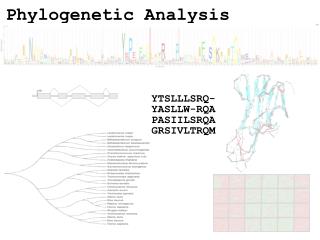
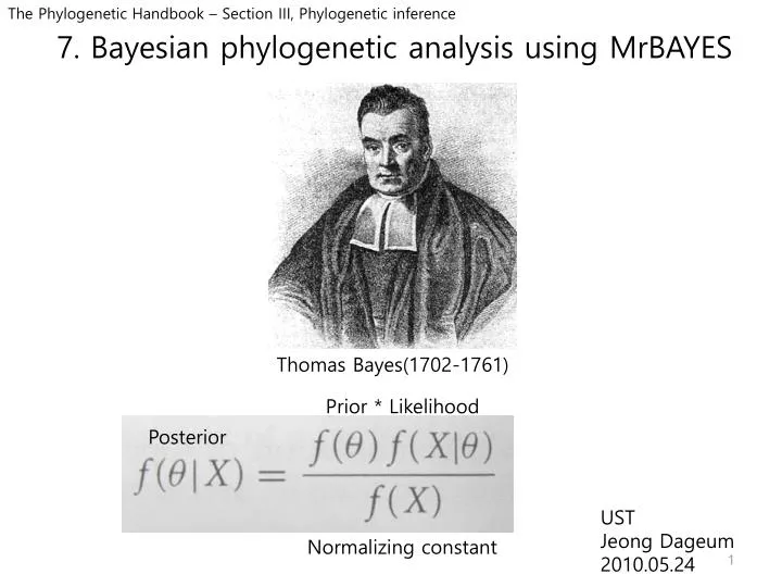
The Phylogenetic Handbook – Section III, Phylogenetic inference. 7. Bayesian phylogenetic analysis using MrBAYES. Thomas Bayes (1702-1761). Prior * Likelihood. Posterior. UST Jeong Dageum 2010.05.24. Normalizing constant. 7. 1 Introduction 7.2 Bayesian phylogenetic inference

E N D
The Phylogenetic Handbook – Section III, Phylogenetic inference 7. Bayesian phylogenetic analysis using MrBAYES Thomas Bayes(1702-1761) Prior * Likelihood Posterior UST JeongDageum 2010.05.24 Normalizing constant
7. 1 Introduction 7.2 Bayesian phylogenetic inference 7.3 Markov chain Monte Carlo sampling 7.4 Burn-in, mixing and convergence 7.5 Metropolis coupling 7.6 Summarizing the results 7.7 An introduction to phylogenetic models 7.8 Bayesian model choice and model averaging 7.9 Prior probability distribution
7.1 Introduction Next year’s world championships in ice hockey? Sweden?!!!! 15 years 1 of 7 countries 1:7 or 0.14 2 gold medal 2:15 or 0.13 Final? Semifinal? Russia, Canada, Finland, Czech Republic, Sweden, Slovakia, United States: 7
7.1 Introduction Bayesianapproach: Bayesian inference is just a mathematical formalization of a decision process that most of us use without reflecting on it Prior * Likelihood Posterior Normalizing Constant
7.1 Introduction Forward probability 50: 50 ? ? Converse ! ? a, b W ball proportion : P B ball proportion: 1-p
7.1 Introduction We know a and b, then What is the probability of a particular value of p? f(p |a,b) = ? : Reverse probability problem Need Prior beliefs about the value of p
7.1 Introduction Box 7.1 Probability distributions – [Considering Prior] [Probability mass function]: a function describing the probability of a discrete Random variable (ex: Dice) [Probability density function]: For a continuous variable, the equivalent function The value of this function is not a probability Exponential distribution: A better choice for a vague prior on branch lengths
7.1 Introduction Box 7.1 Probability distributions – [Considering Prior] Gamma distribution: 2 parameters (shape parameter α, scale parameter β Small value of α: the distribution is L-shaped And the variance is large High value of α: similar to normal distribution The beta distribution The beta distribution denoted Beta (α1, α2) Describes the probability on two proportions, which are associated with the weight parameters.
7.1 Introduction Posterior probability distribution Bayes’ theorem We can calculate f(a,b|p) We can specify f(p) How do we calculate f(a,b)? To integrate over All possible values of p - > Denominator is a normalizing constant
7.2 Bayesian phylogenetic inference Likelihood * Prior P(Data |Tree)P (Tree) P(Tree |Data) = P (Data) Posterior Normalizing constant
7.2 Bayesian phylogenetic inference X: the matrix of aligned sequences Θ: topology, branch length, model.. Θ = (τ: topology parameter υ: branch lengths on the tree) substitution model parameters to be considered (Jukes Cantor substitution model) X(Data) : fixed, Θ(parameter): Random
7.2 Bayesian phylogenetic inference Each cell Summarized all joint probabilities along one axis of the table, we obtain the marginal probabilities for the corresponding parameter. Parameter space It corresponds to a particular set of branch lengths on that topology [Bayesian inference: there is no need to decide on the parameters of interest before performing the analysis]
7.3 Markov chain Monte Carlo sampling [For parameter sampling] • Markov chain Monte Carlo steps • Start an arbitrary point (θ) • Make a small random move (to θ*) • Calculate height ration (r) of new state (to θ*) to old state (θ) • r>1: new state accepted • r<1: new state accepted with probability r • if new state rejected, stay in old state • 4. Go to step 2 f (θ|θ*) ) (Prior ratio) (likelihood ratio) (proposal ratio)
7.3 Markov chain Monte Carlo sampling Box 7.2 Proposal mechanism – To change continuous variables Proposal step Acceptance/Rejection step [Sliding window proposal] ω: tuning parameter Large: more radical proposal & lower acceptance rates Small: more modest changes & higher acceptance rate [Normal proposal] (similar to the above one) σ2: Determine how drastic the new proposals are and how often they will be accepted [Multiplier proposal] [The beta and Dirichlet proposal] σ2: Determine how drastic the new proposals are and how often they will be accepted
7.4 Burn-in, mixing and convergence – [about performance of an MCMC run] * Trace plot * To confirm convergence * Mixing behavior Discard
7.4 Burn-in, mixing and convergence The mixing behavior of a Metropolis sampler can be adjusted using its tuning parameter ω is too small, The proposal will be accepted well Takes long time to cover the all region Poor mixing ω is too large, The proposal will be rejected well Takes long time to cover the all region Poor mixing ω is an intermediate value, Moderate acceptance rates Good mixing
7.4 Burn-in, mixing and convergence • Convergence diagnostics help determine the quality of a sample from the posterior. • 3 different types of diagnostics • (1) Examining autocorrelation times, effective sample sizes, • and other measures of the behavior of single chains • (2) Comparing samples from successive time segments of a single chain • (3) Comparing samples from different runs. • => In Bayesian MCMC sampling of phylogenetic problems, • the tree topology is typically the most difficult parameter to sample from • The approach to solve this problem is to focus on split frequencies instead. • A split is a partition of the tips of the tree into two non-overlapping sets; • To calculate the average standard deviation of the split frequencies. • Potential Scale Reduction Factor(PSRF) • PSRF compares the variance among runs with the variance within runs. • As the chains converge, the variances will become more similar • and the PSRF will approach 1.o
7.5 Metropolis coupling – [To activate the mixing] Cold chain, Hot chain • When: Difficult of impossible to achieve convergence • Metropolis coupling: A General technique to improve mixing * An incremental heating scheme T = 1/ 1 + λi where i∈{ 0,1,…k} for k heated chains, with i=0 for the cold chain, and λ is the temperature factor ( intermediate value of λ works best)
7.6 Summarizing the results Stationary phase of the chain/ Adequate sample > To compute an estimate of the marginal posterior distribution > Summarized using statistics * Bayesian statisticians : 95% credibility interval. The posterior distribution on topology and branch lengths is more difficult to summarize efficiently. * To illustrate the topological variance in posterior -> Estimated number of topologies in various credible sets. * To give the frequencies of the most common splits => A majority rule consensus tree • *The sampled branch lengths are • even more difficult to summarize adequately. • To display the distribution of branch length values separately • To pool the branch length samples that correspond to the same split
7.7 An introduction to phylogenetic models • Phylogenetic model: • A Tree model • Unrooted / rooted model, • Strict / relaxed clock tree model • 2) A substitution model The substitution model, Q matrices The general time-reversible(GTR) model * Factor πi: corresponds to the stationary state frequency of the receiving state * Factor rij,: determines the intensity of the exchange between pairs of states, controlling for the stationary state frequencies
7.8 Bayesian model choice and model averaging * Bayes’ theorem The probability of the data given the chosen model after we have integrated out all parameters: normalizing constant ( model likelihood) Prior Bayes factor • * Bayes factor comparisons are truly flexible. • - Unlike likelihood ratio tests, No requirement for the models to be nexted • Unlike Akaike Information Criterion, Bayesian Information Criterion(confusingly named) • no need to correct for the number of parameters in the model. • To estimate the model likelihood-> Use harmonic means in the MCMC run.
7.9 Prior probability distributions – cautionary notes. The priors : negligible influence on the posterior distribution The Bayesian approach typically handles weak data quite well. But when the data are weak, Extremely low likelihoods that attract the chain. ;;;
Schematic overview of the models implemented in MrBayes3. Each box gives the available settings in normal font and then the program commands and coommand options needed to invoke those settings in italics
PRACTICE 7.10 Introduction to Mrbayes 7.10.1 Acquiring and installing the program 7.10.2 Getting started 7.10.3 Changing the size of the Mrbayes window 7.10.4 Getting help
PRACTICE 7.11 A simple analysis 7.11.1 Quick start version 7.11.2 Getting data into Mrbayes 7.11.3 Specifying a model 7.11.4 Setting the priors 7.11.5 Checking the model 7.11.6 Setting up the analysis 7.11.7 Running the analysis 7.11.8 When to stop the analysis 7.11.9 Summarizing samples of substitution model parameters 7.11.10 Summarizing samples of trees and branch lengths
PRACTICE 7.12 Analyzing a partitioned data set simple analysis 7.12.1 Getting mixed data into Mrbayes 7.12.2 Dividing the data into partitions 7.12.3 Specifying a partitioned model 7.12.4 Running the analysis 7.12.5 Some practical advice