Download

1 / 33
430 likes | 1k Views
Chapter 5 Transient and Steady State Response. “I will study and get ready and someday my chance will come” Abraham Lincoln. Transient vs Steady-State. The output of any differential equation can be broken up into two parts,

E N D
Chapter 5 Transient and Steady State Response “I will study and get ready and someday my chance will come” Abraham Lincoln
Transient vs Steady-State • The output of any differential equation can be broken up into two parts, • a transient part (which decays to zero as t goes to infinity) and • a steady-state part (which does not decay to zero as t goes to infinity). Either part might be zero in any particular case.
Prototype systems 1st Order system 2nd order system Agenda: transfer function response to test signals impulse step ramp parabolic sinusoidal
1st order system Impulse response Step response Ramp response Relationship between impulse, step and ramp Relationship between impulse, step and ramp responses
1st Order system Prototype parameter: Time constant Relate problem specific parameter to prototype parameter. Parameters: problem specific constants. Numbers that do not change with time, but do change from problem to problem. We learn that the time constant defines a problem specific time scale that is more convenient than the arbitrary time scale of seconds, minutes, hours, days, etc, or fractions thereof.
Transient vs Steady state Consider the impulse, step, ramp responses computed earlier. Identify the steady state and the transient parts.
Consider the impulse, step, ramp responses computed earlier. Identify the steady state and the transient parts. 1st order system Impulse response Step response Ramp response Relationship between impulse, step and ramp Relationship between impulse, step and ramp responses Compare steady-state part to input function, transient part to TF.
2nd order system • Over damped • (two real distinct roots = two 1st order systems with real poles) • Critically damped • (a single pole of multiplicity two, highly unlikely, requires exact matching) • Underdamped • (complex conjugate pair of poles, oscillatory behavior, most common) • step response
2nd Order System Prototype parameters: undamped natural frequency, damping ratio Relating problem specific parameters to prototype parameters
Transient vs Steady state Consider the step, responses computed earlier. Identify the steady state and the transient parts.
2nd order system • Over damped • (two real distinct roots = two 1st order systems with real poles) • Critically damped • (a single pole of multiplicity two, highly unlikely, requires exact matching) • Underdamped • (complex conjugate pair of poles, oscillatory behavior, most common) • step response
Use of Prototypes Too many examples to cover them all We cover important prototypes We develop intuition on the prototypes We cover how to convert specific examples to prototypes We transfer our insight, based on the study of the prototypes to the specific situations.
Transient-Response Spedifications • Delay time, td: The time required for the response to reach half the final value the very first time. • Rise time, tr: the time required for the response to rise from • 10% to 90% (common for overdamped and 1st order systems); • 5% to 95%; • or 0% to 100% (common for underdamped systems); • of its final value • Peak time, tp: • Maximum (percent) overshoot, Mp: • Settling time, ts
Derived relations for 2nd Order Systems See book for details. (Pg. 232) Allowable Mp determines damping ratio. Settling time then determines undamped natural frequency. Theory is used to derive relationships between design specifications and prototype parameters. Which are related to problem parameters.
Chapter 5 Homework B problems: 1, 2, 3, 7, do one of the following 9, 10, 11, 27 15, R-H problems, 23, 24, 25, 26, 28, 30, 31, 32
Example: Figure 5-5 Choose physical parameters to achieve a Rise time of .5 seconds Maximum overshoot of 10% 2% settling time of 1.3 seconds Relate physical parameters to prototype parameters. Use prototype relationships. Three requirements, two parameters. See also example 5-2, pg 236-237
Higher order system • PFEs have linear denominators. • each term with a real pole has a time constant • each complex conjugate pair of poles has a damping ratio and an undamped natural frequency. • Read section 5-4
What block diagram? Rational functions are ratios of polynomials. PFE for step input and only distinct real poles. PFE for step input complex roots. PFE for step input and repeated real or complex roots.
Poles of C(s) come from a) TF or b) input function Real Poles in LHP produce decaying exponentials. Complex Poles in LHP produce decaying sinusoids. Simple pole at origin produce step functions. Simple complex poles on imaginary axis produce sinusoids. Multiple poles on imaginary axis produce unbounded terms. Any poles in RHP produce unbounded terms. TF of Stable systems have poles only in LHP. CL poles that are located far from the imaginary axis have real parts that are large negative. These poles decay to zero very fast. Dominant poles produce the terms that dominate the response. Close to imaginary axis, with large residues.
Routh’s Stability Criterion How do we determine stability without finding all poles? Actual poles provide more info than is needed. All we need to know if any poles are in LHP. Routh’s stability criterion (Section 5-7). What values of K produce a stable system?
Derivative Control Action Read at bottom of pg 285-286.
Steady State Errors Bode Form
Steady State Errors-cont. Bode Form Now compute ess for N = 0, 1, 2 and R(s) = 1/s, 1/s2, 1/s3
Steady State Errors-cont. Now compute ess for N = 0, 1, 2 and R(s) = 1/s, 1/s2, 1/s3 Type 1 (=N) systems. Type 2 (=N) systems. Type 3 (=N) systems. Steady state error table, pg. 293, FE Reference manual, notice differences.