3D SPECTROSCOPY OF HERBIG HARO OBJECTS

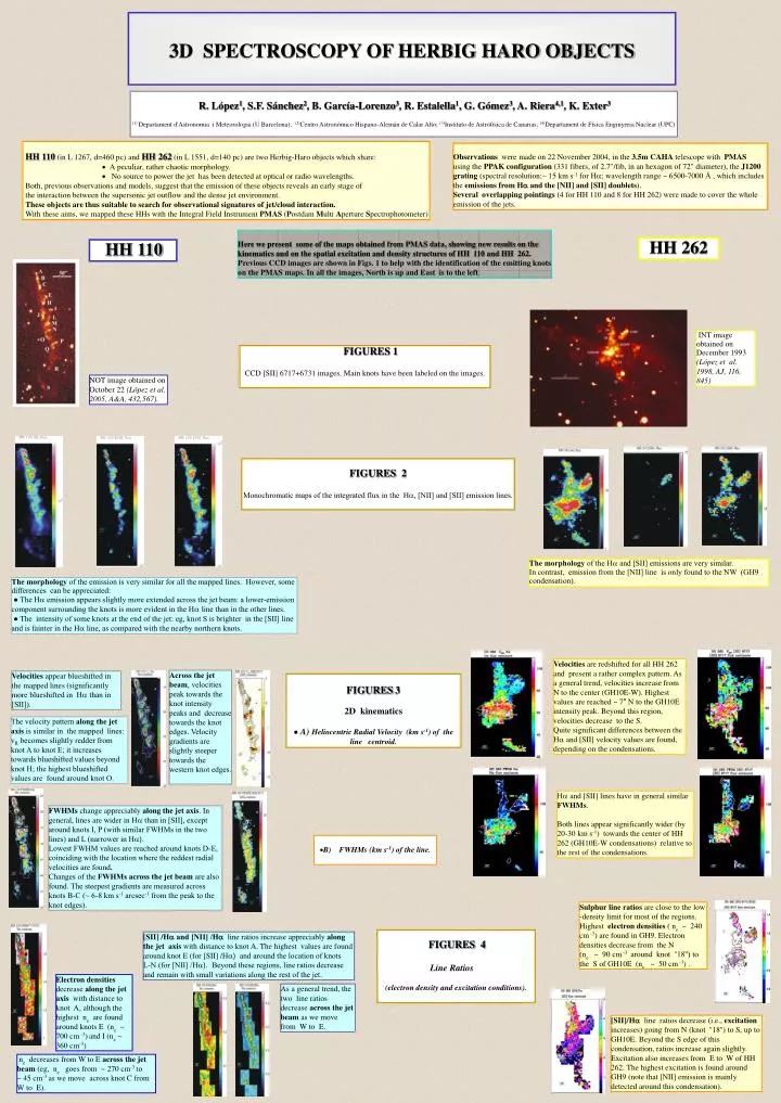
1. 3D SPECTROSCOPY OF HERBIG HARO OBJECTS HH 110 (in L 1267, d=460 pc)and HH 262 (in L 1551, d=140 pc) are two Herbig-Haro objects which share: ·A peculiar, rather chaotic morphology. · No source to power the jet has been detected at optical or radio wavelengths. Both, previous observations and models, suggest that the emission of these objects reveals an early stage of the interaction between the supersonic jet outflow and the dense jet environment. These objects are thus suitable to search for observational signatures of jet/cloud interaction. With these aims, we mapped these HHs with the Integral Field Instrument PMAS (Postdam Multi Aperture Spectrophotometer) Observations were made on 22 November 2004, in the 3.5m CAHA telescope with PMAS using the PPAK configuration (331 fibers, of 2.7"/fib, in an hexagon of 72" diameter), the J1200 grating (spectral resolution:~ 15 km s-1 for H; wavelength range ~ 6500-7000 Å , which includes the emissions from Hand the [NII] and [SII] doublets). Several overlapping pointings (4 for HH 110 and 8 for HH 262) were made to cover the whole emission of the jets. Here we present some of the maps obtained from PMAS data, showing new results on the kinematics and on the spatial excitation and density structures of HH 110 and HH 262. Previous CCD images are shown in Figs. 1 to help with the identification of the emitting knots on the PMAS maps. In all the images, North is up and East is to the left. R. López1, S.F. Sánchez2, B. García-Lorenzo3, R. Estalella1, G. Gómez3, A. Riera4,1, K. Exter3 (1) Departament d'Astronomia i Meteorologia (U.Barcelona); (2)Centro Astronómico Hispano-Alemán de Calar Alto; (3)Instituto de Astrofísica de Canarias; (4)Departament de Física Enginyeria Nuclear (UPC) HH 262 HH 110 INT image obtained on December 1993 (López et al. 1998, AJ, 116, 845) FIGURES 1 CCD [SII] 6717+6731 images. Main knots have been labeled on the images. NOT image obtained on October 22 (López et al. 2005, A&A, 432,567). FIGURES 2 Monochromatic maps of the integrated flux in the H, [NII] and [SII] emission lines. The morphology of the H and [SII] emissions are very similar. In contrast, emission from the [NII] line is only found to the NW (GH9 condensation). The morphology of the emission is very similar for all the mapped lines. However, some differences can be appreciated: ● The H emission appears slightly more extended across the jet beam: a lower-emission component surrounding the knots is more evident in the Hline than in the other lines. ● The intensity of some knots at the end of the jet: eg, knot S is brighter in the [SII] line and is fainter in the H line, as compared with the nearby northern knots. Velocities are redshifted for all HH 262 and present a rather complex pattern. As a general trend, velocities increase from N to the center (GH10E-W). Highest values are reached ~ 7" N to the GH10E intensity peak. Beyond this region, velocities decrease to the S. Quite significant differences between the H and [SII] velocity values are found, depending on the condensations. Across the jet beam, velocities peak towards the knot intensity peaks and decrease towards the knot edges. Velocity gradients are slightly steeper towards the western knot edges. Velocities appear blueshifted in the mapped lines (significantly more blueshifted in Hthan in [SII]). FIGURES3 2D kinematics ● A) Heliocentric Radial Velocity (km s-1) of the line centroid. The velocity pattern along the jet axis is similar in the mapped lines: vR becomes slightly redder from knot A to knot E; it increases towards blueshifted values beyond knot H; the highest blueshifted values are found around knot O. Hand [SII] lines have in general similar FWHMs. Both lines appear significantly wider (by 20-30 km s-1) towards the center of HH 262 (GH10E-W condensations) relative to the rest of the condensations. FWHMs change appreciably along the jet axis. In general, lines are wider in Hthan in [SII], except around knots I, P (with similar FWHMs in the two lines) and L (narrower in H). Lowest FWHM values are reached around knots D-E, coinciding with the location where the reddest radial velocities are found. Changes of the FWHMs across the jet beam are also found. The steepest gradients are measured across knots B-C (~ 6-8 km s-1 arcsec-1 from the peak to the knot edges). • B) FWHMs (km s-1) of the line. Sulphur line ratios are close to the low -density limit for most of the regions. Highest electron densities ( ne ~ 240 cm -3) are found in GH9. Electron densities decrease from the N (ne ~ 90 cm -3 around knot ''18'') to the S of GH10E (ne ~ 50 cm -3) . FIGURES 4 Line Ratios (electron density and excitation conditions). [SII] /Hand[NII] /H line ratios increase appreciably along the jet axis with distance to knot A. The highest values are found around knot E (for [SII] /H) and around the location of knots L-N (for [NII] /H). Beyond these regions, line ratios decrease and remain with small variations along the rest of the jet. Electron densities decrease along the jetaxis with distance to knot A, although the highest ne are found around knots E (ne ~ 700 cm -3)and I (ne ~ 360 cm-3) . As a general trend, the two line ratios decrease across the jetbeam as we move from W to E. [SII]/H line ratios decrease (i.e., excitation increases) going from N (knot ''18'') to S, up to GH10E. Beyond the S edge of this condensation, ratios increase again slightly. Excitation also increases from E to W of HH 262. The highest excitation is found around GH9 (note that [NII] emission is mainly detected around this condensation). ne decreases from W to E across the jetbeam (eg, ne goes from ~ 270 cm-3 to ~ 45 cm-3 as we move across knot C from W to E).