Sampling issues

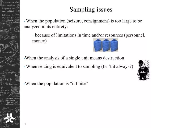
1. Sampling issues • When the population (seizure, consignment) is too large to be analyzed in its entirety: • because of limitations in time and/or resources (personnel, money) • When the analysis of a single unit means destruction • When seizing is equivalent to sampling (Isn’t it always?) • When the population is “infinite”

2. What is sampled? • Drugs (pills, plastic bags, capsules, phials) • Bank-notes and coins • CD-ROMs • Crops (suspected cannabis) • Individuals • Glass • Fibres

3. Objectives of sampling • To do forensic analysis in particular cases • To establish data bases (reference material) for use with evidence evaluation • For quality assurance reasons

4. Two “general” cases • The population is expected to be (large and) heterogeneous • Difficult to make prior assumptions about population parameters • Sample size must usually be large (…to reflect the heterogeneity) •  Normal approximations are valid and sample size determination can be done with the “frequentist” approach • The population is expected to be homogeneous • Easier to make prior assumption about population parameters • Sample size needs not to be large (e.g. if we are 100 % certain that all elements in the population are of the same kind, we only need to sample one unit) • Bayesian approach to sample size determination is more attractable.

5. The heterogeneous case • Undesirable for forensic analysis in particular cases • Expected when data bases are to be established • Sampling of individuals, glass, fibres etc. • Should be carried out with careful use of knowledge from survey theory: • Comparison of frame population with true population • Choice of sampling design (simple random sampling, stratified sampling, cluster sampling,…) • Efficient prevention and post-handling of non-response

6. The homogeneous case • Main “Objective” of the current presentation • Required for efficient sampling in daily case-work • Sampling of drug pills, bank-notes, CD-ROMs etc. for further analysis • General desire: To keep the sample size very small (5-10 units) • Sampling under experimental conditions for inference about proportions • General desire: To keep the sample size as small as possible

7. Some examples from drug sampling 1. Homogeneity expected from visual inspection and experience Consider a case with a seizure of 5000 pills, all of the same colour (blue), form (circular) and printing (e.g. the Mitsubishi trade mark) The forensic scientist would say “this is a seizure of Ecstasy pills”

8. Some examples from drug sampling • So, what do we know about blue pills (supposed to be Ecstasy)? • Consider historical cases with blue pills • Group the cases into M clusters with respect to another parameter, e.g. the print on the pill. • Find an estimate of the prior distribution for the proportion  of Ecstasy pills among blue pills. • Nordgaard A. (2006) Quantifying experience in sample size determination for drug analysis of seized drugs. Law, Probability and Risk 4: 217-225

9. Some examples from drug sampling Use a generic beta prior for the proportion  of Ecstasy pills in the current seizure:

10. Some examples from drug sampling Use the grouped data to estimate the parameters 1and 2 of this beta prior. This can be done by the maximum likelihood method using that the probability of obtaining xiEcstasy pills in cluster i is where “    ” stands for rounding downwards to nearest integer Hypergeometric distribution The likelihood function is thus

11. Some examples from drug sampling The obtained point estimates of 1and 2 can be assessed with respect to bias and variance using bootstrap resampling. In Nordgaard (2006) original point estimates of 1and 2 for historical cases of blue pills at SKL are Bias adjusted estimates are and upper 90% confidence limits for the true values of 1and 2 are

12. Some examples from drug sampling Now, assume the forthcoming sample of n units will consist entirely of Ecstasy pills. (Otherwise the case will be considered “non-standard”) The sample size is determined so that the posterior probability of  being higher than a certain proportion, say 50 %, is at least say 99% (referred to as 99% credibility) For large seizures the posterior distribution of  given all n sample units consist of Ecstasy is also beta:

13. Some examples from drug sampling Thus we solve for n where 1and 2 are replaced by their (adjusted) point estimates or upper confidence limits.

14. Some examples from drug sampling For the above case we find that with the bias-adjusted point estimates the required sample size is at least 3 and with the upper confidence limits used instead (i.e with 0.062 and 0.262) the required sample size is at least 4 There are in general no large differences between different choices of estimated parameters, nor between different colours of Ecstasy pills. A general sampling rule of n =5 can therefore be used to state with 99% credibility that at least 50% of the seizure consists of Ecstasy pills. For a higher proportion, a sample size around 12 appears to be satisfactory.

15. Some examples from drug sampling For smaller seizures it is more wise to rephrase the requirement in terms of the number of Ecstasy units in the non-sampled part of the seizure. The posterior beta distribution is then replaced with a beta-binomial distribution.

16. Some examples from drug sampling 2. Homogeneity stated upon inspection only Consider now a case with a (large) seizure of drug pills of which the forensic scientist cannot directly suspect the contents. Visual inspection  All pills seem to be identical Can we substitute the “experience” from the Ecstasy case?

17. Some examples from drug sampling UV-lightning Pills can be inspected under UV light. The fluorescence differs between pills with different chemical composition and looking at a number of pills under UV light would thus reveal (to greatest extent) heterogeneity. Uncertainty of this procedure lies mainly with the person who does the inspection  Experiment required!

18. Some examples from drug sampling Assume a prior g( ) for the proportion of pills in the seizure that contains a certain (but possibly unknown) illicit drug. For sake of simplicity, assume that pills may be of two kinds (the illicit drug or another substance). Let Y be a random variable associated with the inspection such that

19. Some examples from drug sampling Relevant case is Y = 0 (Otherwise the result of the UV-inspection has rejected the assumption of homogeneity.) Now, is the false positive probability as a function of  (if a positive result means that no heterogeneity is detected) while is the true positive probability

20. Some examples from drug sampling The prior g can be updated using this information (when available) Note that an non-informative prior (i.e. g( )  1 ; 0    1 can be used. The updated prior (i.e. the posterior upon UV-inspection) can then be used analogously to the previous case (Ecstasy)

21. Some examples from drug sampling • Example Experiment (conducted at SKL) • 8 types of pills with different substances were used to form 9 different mixes (i.e. in two proportions) of 2 types of pills. • Each mix was prepared by randomly shuffling 100 pills with the current proportions on a tray that was put under UV-light • 10 case-workers made inspections in random order such that a total of 114-117 inspections were made for each mix

22. Some examples from drug sampling Results:

23. Some examples from drug sampling Data can be illustrated by plotting estimated probabilities for Y = 0 vs.  Linear interpolation gives

24. Some examples from drug sampling To avoid the vertices at  = 0.02, 0.20, 0.80 and 0.98, the linearly interpolated values are smoothed using a Kernel function: where K(x) is a symmetric function integrating to one over its support.

25. Some examples from drug sampling Now, the prior can be updated using this smoothed function as an estimate of , i.e. (With a non-informative prior g, this simplifies into )

26. Some examples from drug sampling Comparison of the non-informative prior and the updated prior

27. Some examples from drug sampling Now, let x be the number of illicit drug pills found in a sample of n pills. Analogously with the Ecstasy case n should be determined so that if x = n a 99% credible lower limit for  is 50% (or even higher). With the updated prior derived the following table of posterior probabilities is obtained Thus, a sample size of n =3 units is satisfactory. Slightly higher values may be recommended due to the limits of the experiment