Download
1 / 29
290 likes | 360 Views
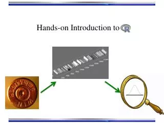
Hands-on Introduction to R. Why Leaning Programing?. We live in oceans of data. Computers are essential to record and help analyse it. Competent scientists speak C/C++, Java, MATLAB, Python, Perl, R and/or Mathematica

E N D
Why Leaning Programing? • We live in oceans of data. Computers are essential to record and help analyse it. • Competent scientists speak C/C++, Java, MATLAB, Python, Perl, R and/or Mathematica • Data collection and analysis very important in Forensic Science since NAS 2009 • Using the above languages, codes can easily be made available for review/discovery
Getting a computer to do anything useful • All machines understand is on/off! • High/low voltage • High/low current • High/low charge • 1/0 binary digits (bits) • To make a computer do anything, you have to speak machine language to it: 000000 00001 00010 00110 00000 100000 Add 1 and 2. Store the result.Wikipedia
Getting a computer to do anything useful • Machine language is not intuitive and can vary a great deal over designs • The basic operations operations however are the same, e.g.: • Move data here • Combine these values • Store this data • Etc. • “Human readable” language for basic machine operations: assembly language
Getting a computer to do anything useful • Assembly is still cumbersome for (most) humans A machine encoding 10110000 01100001 Assembly MOV AL, 61h Move the number 97 over to “storage area” AL
Getting a computer to do anything useful • Better yet is a more “Englishy”, “high-level” language • Enter: C, C++, Fortran, Java, … • Higher level languages like these are translated (“compiled”) to machine language • Not exactly true for Java, but it’s something analogous…
Getting a computer to do anything useful • Even more “Englishy”and “high-level” are interpreted languages • Enter: R MATLAB, Perl, Python, Mathematica, Maple, … • The “code” of these languages are “interpreted” as commands by a program that is already running • They make many assumptions behind the scenes • Much easier to program with • Much slower than compiled languages
Why ? • R is not a black box! • Codes available for review; totally transparent! • R maintained by a professional group of statisticians, and computational scientists • From very simple to state-of-the-art procedures available • Very good graphics for exhibits and papers • R is extensible (it is a full scripting language) • Coding/syntax similar to Python and MATLAB • Easy to link to C/C++ routines
Why ? • Where to get information on R : • R: http://www.r-project.org/ • Just need the base • RStudio: http://rstudio.org/ • A great IDE for R • Work on all platforms • Sometimes slows down performance… • CRAN: http://cran.r-project.org/ • Library repository for R • Click on Search on the left of the website to search for package/info on packages
Finding our way around R/RStudio Script Window Command Line
Handy Commands: • Basic Input and Output Numeric input x <- 4 variables: store information :Assignment operator x <- “text goes in quotes” Text (character) input
Handy Commands: • Get help on an R command: • If you know the name: ?command name • ?plot brings up html on plot command • If you don’t know the name: • Use Google (my favorite) • ??key word
Handy Commands: • R is driven by functions: func(arguement1, argument2) input to function goes in parenthesis function name function returns something; gets dumped into x x <- func(arg1, arg2)
Handy Commands: • Input from Excel • Save spreadsheet as a CSV file • Use read.csv function • Needs the path to the file Mac e.g.: "/Users/npetraco/latex/papers/data.csv” Windows e.g.: “C:\Users\npetraco\latex\papers\data.csv” *Exercise: basicIO.R
Handy Commands: • Matrices: X • X[,1] returns column 1 of matrix X • X[3,] returns row 3 of matrix X • Handy functions for data frames and matrices: • dim, nrow, ncol, rbind, cbind • User defined functions syntax: • func.name <- function(arguements) { • do something • return(output) • } • To use it: func.name(values)
Handy Commands: • User defined function example: • Compute the intensities of the Planck distribution • Let the user input a Temperature • Let the user input endpoint. Assume it is in nm • Careful here. Make sure wavelength units are consistent with the other constants. • What is the “easiest” thing to do??
First Thing: Look at your Data • Explore the Glass dataset of the mlbench package • Source (load) all_data_source.R • *visualize_with_plots.r • Scatter plots: plot any two variables against each other
First Thing: Look at your Data • Pairs plots: do many scatter plots at once
First Thing: Look at your Data • Histograms: “bin” a variable and plot frequencies
First Thing: Look at your Data • Histograms conditioned on other variables: use lattice package RIs Conditioned on glass group membership
First Thing: Look at your Data • Probability density plots: also needs lattice
First Thing: Look at your Data • Empirical Probability Distribution plots: also called empirical cumulative density
First Thing: Look at your Data • Box and Whiskers plots: range possible outliers possible outliers 25th-%tile 1st-quartile 75th-%tile 3rd-quartile median 50th-%tile RI
Visualizing Data • Note the relationship:
First Thing: Look at your Data • Box and Whiskers plots: Box-Whiskers plots for actual variable values Box-Whiskers plots for scaled variable values
Confidence Intervals • A confidence interval (CI) gives a range in which a true population parameter may be found. • Specifically,(1 – a)×100% CIs for a parameter, constructed from a random sample (of a given sample size), will contain the true value of the parameter approximately (1 – a)×100% of the time. • Different from tolerance and prediction intervals
Confidence Intervals • Caution: IT IS NOT CORRECT to say that there a (1 - a)×100% probability that the true valueof a parameter is between the bounds of any given CI. Take a sample. Compute a CI. Here 90% of the CIs contain the true value of the parameter Graphical representation of 90% CIs is for a parameter: true value of parameter
Confidence Intervals • Construction of a CI for a mean depends on: • Sample size n • Standard error for means • Level of confidence 1- • is significance level • Use to compute tc-value • (1-)×100% CI for population mean using a sample average and standard error is:
Confidence Intervals • Compute a 99% confidence interval for the mean using this sample set: (a/2=0.005) tc = 3.17 Putting this together: [1.52005 - (3.17)(0.00001), 1.52005 + (3.17)(0.00001)] 99% CI for sample = [1.52002, 1.52009] *Try out confidence_intervals.R