Download
1 / 35
350 likes | 505 Views
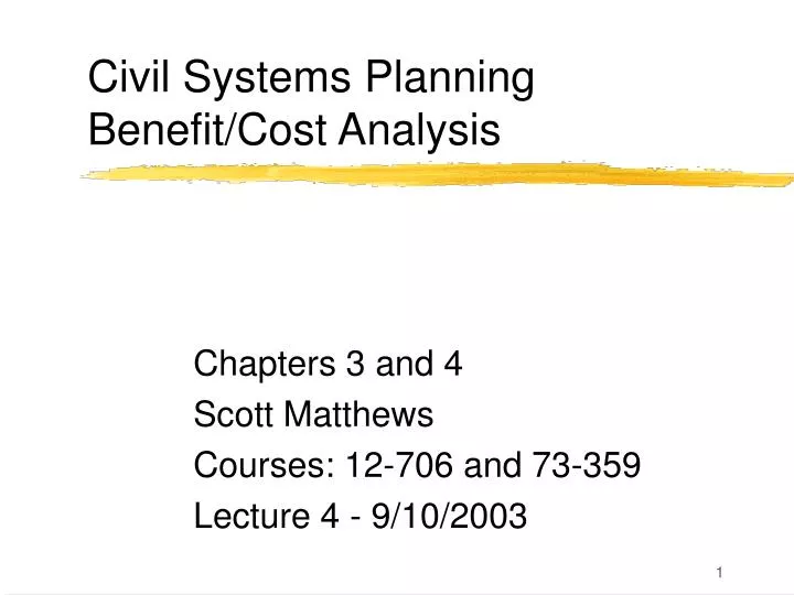
Civil Systems Planning Benefit/Cost Analysis. Chapters 3 and 4 Scott Matthews Courses: 12-706 and 73-359 Lecture 4 - 9/10/2003. Price. A. B. P*. 0 1 2 3 4 Q*. Quantity. Recap: Net Benefits. A. B.

E N D
Civil Systems PlanningBenefit/Cost Analysis Chapters 3 and 4 Scott Matthews Courses: 12-706 and 73-359 Lecture 4 - 9/10/2003
Price A B P* 0 1 2 3 4 Q* Quantity Recap: Net Benefits A B • Amount ‘paid’ by society at Q* is P*, so total payment is B to receive (A+B) total benefit • Net benefits = (A+B) - B = A = consumer surplus (benefit received - price paid) 12-706 and 73-359
Short Run vs. Long Run Cost • Short term / short run - some costs fixed • In long run, “all costs variable” • Difference is in ‘degree of control of plans’ • Generally say we are ‘constrained in the short run but not the long run’ • So TC(q) < = SRTC(q) 12-706 and 73-359
BCA Part 2: CostWelfare Economics Continued The upper segment of a firm’s marginal cost curve corresponds to the firm’s SR supply curve. Again, diminishing returns occur. Price At any given price, determines how much output to produce to maximize profit Supply=MC AVC Quantity 12-706 and 73-359
Supply/Marginal Cost Notes Demand: WTP for each additional unit Supply: cost incurred for each additional unit Supply=MC Price At any given price, determines how much output to produce to maximize profit P* Q1 Q* Q2 Quantity 12-706 and 73-359
Supply/Marginal Cost Notes Recall: We always want to be considering opportunity costs (total asset value to society) and not accounting costs Supply=MC Price Area under MC is TVC - why? P* Q1 Q* Q2 Quantity 12-706 and 73-359
Market Supply Curves Producer surplus is similar to CS -- the amount over and Above cost required to produce a given output level Changes in PS found the same way as before Supply=MC Price P* PS* P1 PS1 TVC* TVC1 Quantity Q1 Q* Producer Surplus = Economic Profit 12-706 and 73-359
Unifying Cost and Supply • Economists learn “Supply and Demand” • Equilibrium (meeting point): where S = D • In our case, substitute ‘cost’ for supply • Why cost? Need to trade-off Demand • Using MC is a standard method 12-706 and 73-359
Example • Demand Function: p = 4 - 3q • Supply function: p = 1.5q • Assume equilibrium, what is p,q? • In eq: S=D; 4-3q=1.5q ; 4.5q=4 ; q=8/9 • P=1.5q=(3/2)*(8/9)= 4/3 • CS = (0.5)*(8/9)*(4-1.33) = 1.19 • PS = (0.5)*(8/9)*(4/3) = 0.6 12-706 and 73-359
Allocative Efficiency Allocative efficiency occurs when MC = MB (or S = D) S = MC Price b P* D = MB a Q1 Q* Q2 Quantity 12-706 and 73-359
Social Surplus = consumer surplus + producer surplus Losses in Social Surplus are Dead-Weight Losses! P S P* D Q* Q Social Surplus 12-706 and 73-359
Subsidies/Target Pricing Allocative efficiency only achieved when P = social MC. Assume market for corn below in initial eq’m -> what happens when government guarantees PT to farmers? S Price a d PT b P* D c Q* QT Quantity 12-706 and 73-359
Subsidies/Target Pricing At PT, farmers want to supply QT units. But at QT , consumers only want to pay PD . This is effective market price. So PT-PD must be subsidized by government policy. What is change in CS, PS? S Price a d PT b P* PD e D c Q* QT Quantity 12-706 and 73-359
Subsidies/Target Pricing CS increases from aP*b (yellow) to aPDe (yellow+orange). What about PS? S Price a d PT b P* PD e D c Q* QT Quantity 12-706 and 73-359
Subsidies/Target Pricing PS also increases, from P*bc to PTdc. So is overall net benefit to society then positive (since PS and CS both increase)? S Price a d PT b P* PD e D c c Q* QT Quantity 12-706 and 73-359
Subsidies/Target Pricing A cost to society (taxpayers) is the government subsidy - So what is the overall net benefit to society? S Price a d PT b P* PD e D c Q* QT Quantity 12-706 and 73-359
Subsidies/Target Pricing Overall net benefit to society is (Increased CS + Increased PS) - Costs = Orange + Yellow - Grey = Triangle bde (loss!). This is a DWL, increases in CS, PS are transfers! Efficiency Measure: Leakage = Area bde/Area PTdePD Price S a d PT b P* PD e D c Quantity Q* QT 12-706 and 73-359
Changes in Demand • There is a difference in ‘change in quantity demanded’ and a ‘change in demand’. • If (only) the price of good changes • Change in qty demanded - move along D • If something other than price changes (e.g. demand more of good) • Then entire demand curve shifts • Same things true for supply 12-706 and 73-359
Types of Markets • Primary: directly affected by policy • Secondary: indirectly affected • Example: new highway • Primary: commuting, traffic, pollution • Secondary: change in repairs, gas • Efficient markets (as discussed) • Distorted markets: when external effects occur as a result of market • Could be positive or negative 12-706 and 73-359
Benefits in Efficient Market • NSB=DCS+ DPS + Net Gov’t Revenues • Government adds large quantity of good to market to reduce price • Example: surplus food programs • Government intervenes by supplying q’ units into the market • Supply curve moves out (right) - more supplied at each price point 12-706 and 73-359
Surplus Food Example Initial equilibrium at P0, Q0 New eq’m at (lower)P1, (higher) Q1 What is change in CS? S P S+q’ a P0 b P1 D Q Q2 Q0 Q1 12-706 and 73-359
Surplus Food Example Change in CS is P0abP1 (gain) What about PS? S P S+q’ a P0 b P1 D Q Q2 Q0 Q1 12-706 and 73-359
Surplus Food Example Change in PS is P0acP1 (loss) for the ‘original suppliers’ since they still Operate on supply curve ‘S’ What is social surplus? S P S+q’ a P0 b P1 c D Q Q2 Q0 Q1 12-706 and 73-359
Surplus Food Example Social surplus is net gain of CS+PS, Or the triangle abc - what is Net Social Benefit? S P S+q’ a P0 b P1 c D Q Q2 Q0 Q1 12-706 and 73-359
Surplus Food Example Government gains revenue Q2cbQ1, so NSB =Q2cabQ1 S P S+q’ a P0 b P1 c D Q Q2 Q0 Q1 12-706 and 73-359
Monopoly - the real game • One producer of good w/o substitute • Not example of perfect comp! • Deviation that results in DWL • There tend to be barriers to entry • Monopolist is a price setter not taker • Monopolist is only firm in market • Thus it can set prices based on output 12-706 and 73-359
Monopoly - the real game (2) • Could have shown that in perf. comp. Profit maximized where p=MR=MC • Same is true for a monopolist -> she can make the most money where additional revenue = added cost • But unlike perf comp, p not equal to MR 12-706 and 73-359
Monopoly Analysis In perfect competition, Equilibrium was at (Pc,Qc) - where S=D. But a monopolist has a Function of MR that Does not equal Demand So where does he supply? MC Pc Qc MR D 12-706 and 73-359
Monopoly Analysis (cont.) Monopolist supplies where MR=MC for quantity to max. profits (at Qm) But at Qm, consumers are willing to pay Pm! What is social surplus, Is it maximized? MC Pm Pc Qm Qc D MR 12-706 and 73-359
Monopoly Analysis (cont.) What is social surplus? Orange = CS Yellow = PS (bigger!) Grey = DWL (from not Producing at Pc,Qc) thus Soc. Surplus is not maximized Breaking monopoly Would transfer DWL to Social Surplus MC Pm Pc Qm Qc D MR 12-706 and 73-359
Natural Monopoly • Fixed costs very large relative to variable costs • Ex: public utilities (gas, power, water) • Average costs high at low output • AC usually higher than MC • One firm can provide good or service cheaper than 2+ firms • In this case, government allows monopoly but usually regulates it 12-706 and 73-359
Natural Monopoly Faced with these curves Normal monop would Produce at Qm and Charge Pm. We would have same Social surplus. But natural monopolies Are regulated. What are options? a Pm d P* AC b e MC c Qm Q* D MR 12-706 and 73-359
Natural Monopoly Forcing the price P* Means that the social surplus is increased. DWL decreases from abc to dec Society gains adeb a Pm d P* AC b e MC c D Qm Q* Q0 MR 12-706 and 73-359
Monopoly • Other options - set P = MC • But then the firm loses money • Subsidies needed to keep in business • Give away good for free (e.g. road) • Free rider problems • Also new deadweight loss from cost exceeding WTP 12-706 and 73-359
Pricing Strategies • Highway pricing • If price set equal to AC (which is assumed to be TC/q then at q, total costs covered • p ~ AVC: manages usage of highway • p = f(fares, fees, travel times, discomfort) • Price increase=> less users (BCA) • MC pricing: more users, higher price • What about social/external costs? • Might want to set p=MSC 12-706 and 73-359