Data Mining Classification: Basic Concepts, Decision Trees, and Model Evaluation

1. Data Mining Classification: Basic Concepts, Decision Trees, and Model Evaluation Lecture Notes for Chapter 4 By Gun Ho Lee ghlee@ssu.ac.kr Intelligent Information Systems Lab Soongsil University, Korea This material is modified and reproduced based on books and materials of P-N, Ran and et al, J. Han and M. Kamber, M. Dunham, etc

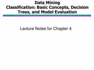
2. Classification: Definition • Given a collection of records (training set ) • Each record contains a set of attributes, one of the attributes is the class. • Find a model for class attribute as a function of the values of other attributes. • Goal: previously unseen records should be assigned a class as accurately as possible. • A test set is used to determine the accuracy of the model. Usually, the given data set is divided into training and test sets, with training set used to build the model and test set used to validate it.

3. Illustrating Classification Task

4. Examples of Classification Task • Predicting tumor cells as benign or malignant • Classifying credit card transactions as legitimate or fraudulent • Classifying secondary structures of protein as alpha-helix, beta-sheet, or random coil • Categorizing news stories as finance, weather, entertainment, sports, etc

5. Classification Techniques • Decision Tree based Methods • Rule-based Methods • Memory based reasoning • Neural Networks • Naïve Bayes and Bayesian Belief Networks • Support Vector Machines

6. categorical categorical continuous class Example of a Decision Tree Splitting Attributes Refund Yes No NO MarSt Married Single, Divorced TaxInc NO < 80K > 80K YES NO Model: Decision Tree Training Data

7. NO Another Example of Decision Tree categorical categorical continuous class Single, Divorced MarSt Married NO Refund No Yes TaxInc < 80K > 80K YES NO There could be more than one tree that fits the same data!

8. Decision Tree Classification Task Decision Tree

9. Refund Yes No NO MarSt Married Single, Divorced TaxInc NO < 80K > 80K YES NO Apply Model to Test Data Test Data Start from the root of tree.

10. Refund Yes No NO MarSt Married Single, Divorced TaxInc NO < 80K > 80K YES NO Apply Model to Test Data Test Data

11. Apply Model to Test Data Test Data Refund Yes No NO MarSt Married Single, Divorced TaxInc NO < 80K > 80K YES NO

12. Apply Model to Test Data Test Data Refund Yes No NO MarSt Married Single, Divorced TaxInc NO < 80K > 80K YES NO

13. Apply Model to Test Data Test Data Refund Yes No NO MarSt Married Single, Divorced TaxInc NO < 80K > 80K YES NO

14. Apply Model to Test Data Test Data Refund Yes No NO MarSt Assign Cheat to “No” Married Single, Divorced TaxInc NO < 80K > 80K YES NO

15. Decision Tree Classification Task Decision Tree

16. Decision Tree Induction • Many Algorithms: • Hunt’s Algorithm (one of the earliest) • CART • ID3, C4.5 • SLIQ,SPRINT

17. General Structure of Hunt’s Algorithm • Let Dt be the set of training records that reach a node t • General Procedure: • If Dt contains records that belong the same class yt, then t is a leaf node labeled as yt • If Dt is an empty set, then t is a leaf node labeled by the default class, yd • If Dt contains records that belong to more than one class, use an attribute test to split the data into smaller subsets. Recursively apply the procedure to each subset. Dt ?

18. Refund Refund Yes No Yes No Cheat=No Marital Status Cheat=No Marital Status Single, Divorced Refund Married Married Single, Divorced Yes No Cheat=No Taxable Income Cheat Cheat=No Cheat=No Cheat=No < 80K >= 80K Cheat=No Cheat Hunt’s Algorithm Cheat=No

19. Tree Induction • Greedy strategy. • Split the records based on an attribute test that optimizes certain criterion. • Issues • Determine how to split the records • How to specify the attribute test condition? • How to determine the best split? • Determine when to stop splitting

20. How to Specify Test Condition? • Depends on attribute types • Nominal • Ordinal • Continuous • Depends on number of ways to split • 2-way split • Multi-way split

21. CarType Family Luxury Sports CarType CarType {Sports, Luxury} {Family, Luxury} {Family} {Sports} Splitting Based on Nominal Attributes • Multi-way split: Use as many partitions as distinct values. • Binary split: Divides values into two subsets. Need to find optimal partitioning. OR

22. Size Small Large Medium Size Size Size {Small, Medium} {Small, Large} {Medium, Large} {Medium} {Large} {Small} Splitting Based on Ordinal Attributes • Multi-way split: Use as many partitions as distinct values. • Binary split: Divides values into two subsets. Need to find optimal partitioning. • What about this split? OR

23. Splitting Based on Continuous Attributes • Different ways of handling • Discretization to form an ordinal categorical attribute • Static – discretize once at the beginning • Dynamic – ranges can be found by equal interval bucketing, equal frequency bucketing (percentiles), or clustering. • Binary Decision: (A < v) or (A  v) • consider all possible splits and finds the best cut • can be more compute intensive

24. Splitting Based on Continuous Attributes

25. Algorithm for Decision Tree Induction • Basic algorithm (a greedy algorithm) • Tree is constructed in a top-down recursive divide-and-conquer manner • At start, all the training examples are at the root • Attributes are categorical (if continuous-valued, they are discretized in advance) • Examples are partitioned recursively based on selected attributes • Test attributes are selected on the basis of a heuristic or statistical measure (e.g., information gain) • Conditions for stopping partitioning • All samples for a given node belong to the same class • There are no remaining attributes for further partitioning –majority voting is employed for classifying the leaf • There are no samples left

26. Tree Induction • Greedy strategy. • Split the records based on an attribute test that optimizes certain criterion. • Issues • Determine how to split the records • How to specify the attribute test condition? • How to determine the best split? • Determine when to stop splitting

27. How to determine the Best Split Before Splitting: 10 records of class 0, 10 records of class 1 Which test condition is the best?

28. How to determine the Best Split • Greedy approach: • Nodes with homogeneous class distribution are preferred • Need a measure of node impurity: Non-homogeneous, High degree of impurity Homogeneous, Low degree of impurity

29. Measures of Node Impurity • Gini Index • Entropy • Misclassification error

30. M0 M2 M3 M4 M1 M12 M34 How to Find the Best Split Before Splitting: A? B? Yes No Yes No Node N1 Node N2 Node N3 Node N4 Gain = M0 – M12 vs M0 – M34

31. Measure of Impurity: GINI • Gini Index for a given node t : (NOTE: p( j | t) is the relative frequency of class j at node t). • Maximum (1 - 1/nc) when records are equally distributed among all classes, implying least interesting information • Minimum (0.0) when all records belong to one class, implying most interesting information

32. Examples for computing GINI P(C1) = 0/6 = 0 P(C2) = 6/6 = 1 Gini = 1 – P(C1)2 – P(C2)2 = 1 – 0 – 1 = 0 P(C1) = 1/6 P(C2) = 5/6 Gini = 1 – (1/6)2 – (5/6)2 = 0.278 P(C1) = 2/6 P(C2) = 4/6 Gini = 1 – (2/6)2 – (4/6)2 = 0.444

33. Splitting Based on GINI • Used in CART, SLIQ, SPRINT. • When a node p is split into k partitions (children), the quality of split is computed as, where, ni = number of records at child i, n = number of records at node p.

34. Binary Attributes: Computing GINI Index • Splits into two partitions • Effect of Weighing partitions: • Larger and Purer Partitions are sought for. B? Yes No Node N1 Node N2 Gini(N1) = 1 – (5/7)2 – (2/7)2= 0.408 Gini(N2) = 1 – (1/5)2 – (4/5)2= 0.320 Ginisplit(Children) = 7/12 * 0.408 + 5/12 * 0.320= 0.371

35. Binary Attributes: Computing GINI Index • Which splitting is preferred ? B? A? No Yes No Yes Node N1 Node N2 Node N1 Node N2 N1 N2 C1 4 2 C2 3 3 Gini=0.486

36. Categorical Attributes: Computing Gini Index • For each distinct value, gather counts for each class in the dataset • Use the count matrix to make decisions Multi-way split Two-way split (find best partition of values)

37. Continuous Attributes: Computing Gini Index • Use Binary Decisions based on one value • Several Choices for the splitting value • Number of possible splitting values = Number of distinct values • Each splitting value has a count matrix associated with it • Class counts in each of the partitions, A < v and A  v • Simple method to choose best v • For each v, scan the database to gather count matrix and compute its Gini index • Computationally Inefficient! Repetition of work.

38. Sorted Values Split Positions Continuous Attributes: Computing Gini Index... • For efficient computation: for each attribute, • Sort the attribute on values • Linearly scan these values, each time updating the count matrix and computing gini index • Choose the split position that has the least gini index

39. Splitting Criteria based on Classification Error • Classification error at a node t : • Measures misclassification error made by a node. • Maximum (1 - 1/nc) when records are equally distributed among all classes, implying least interesting information • Minimum (0.0) when all records belong to one class, implying most interesting information

40. Examples for Computing Error P(C1) = 0/6 = 0 P(C2) = 6/6 = 1 Error = 1 – max (0, 1) = 1 – 1 = 0 P(C1) = 1/6 P(C2) = 5/6 Error = 1 – max (1/6, 5/6) = 1 – 5/6 = 1/6 P(C1) = 2/6 P(C2) = 4/6 Error = 1 – max (2/6, 4/6) = 1 – 4/6 = 1/3

41. Misclassification Error vs Gini A? Yes No Node N1 Node N2 Gini(N1) = 1 – (3/3)2 – (0/3)2= 0 Gini(N2) = 1 – (4/7)2 – (3/7)2= 0.489 Gini(Children) = 3/10 * 0 + 7/10 * 0.489= 0.342 Gini improves !!

42. Misclassification Error vs Gini A? Yes No Node N1 Node N2 Error(N1) = 1 – max(0/3, 3/3) = 0 Error(N2) = 1 – max(4/7, 3/7) = 0.429 Error(Children) = 3/10 * 0 + 7/10 * 0.429= 0.30 Error doesn’t improves !!

43. Alternative Splitting Criteria based on INFO • Entropy at a given node t: (NOTE: p( j | t) is the relative frequency of class j at node t). • Measures homogeneity of a node. • Maximum (log nc) when records are equally distributed among all classes, implying least information • Minimum (0.0) when all records belong to one class, implying most information • Entropy based computations are similar to the GINI index computations

44. P(C1) = 2/6 P(C2) = 4/6 E(2/6, 4/6) = – (2/6) log2 (2/6)– (4/6) log2 (4/6) = 0.92 Examples for computing Entropy P(C1) = 0/6 = 0 P(C2) = 6/6 = 1 E(0, 1) = – 0 log 0– 1 log 1 = – 0 – 0 = 0 P(C1) = 1/6 P(C2) = 5/6 E(1/6, 5/6) = – (1/6) log2 (1/6)– (5/6) log2 (1/6) = 0.65

45. Comparison among Splitting Criteria For a 2-class problem:

46. Decision Tree Training Dataset

47. Output: A Decision Tree for “buys_computer” age? <=30 >40 overcast 30..40 credit rating? student? yes fair excellent no yes no yes no yes

48. Splitting Based on INFO... • Information Gain: Parent Node, p is split into k partitions; ni is number of records in partition i • Measures Reduction in Entropy achieved because of the split. • Choose the split that achieves maximum GAIN value !! • Used in ID3 and C4.5 • Disadvantage: Tends to prefer splits that result in large number of partitions, each being small but pure.

49. Attribute Selection by Information Gain Computation • Class P: 컴퓨터소유 = “yes” • Class N: 컴퓨터 소유 = “no” • E(컴퓨터 소유) = E(p, n) = E(9, 5) =0.940 • Compute the entropy for age: means “age <=30” has 5 out of 14 samples, with 2 yes’es and 3 no’s. Hence Gain(age) = E(컴소유) –E(age) = 0.246 Similarly,

50. Customer ID 1 2 3 4 5 6 7 8 9 10 11 12 13 14 15 16 17 18 19 20 Gender M M M M M M F F F F M M M M F F F F F F Car Type Family Sports Sports Sports Sports Sports Sports Sports Sports Luxury Family Family Family Luxury Luxury Luxury Luxury Luxury Luxury Luxury Shirt Size Small Medium Medium Large Extra Large Extra Large Small Small Medium Large Large Extra Large Medium Extra Large Small Small Medium Medium Medium Large Class C0 C0 C0 C0 C0 C0 C0 C0 C0 C0 C1 C1 C1 C1 C1 C1 C1 C1 C1 C1 DataSet Not predictive attribute due to its unique value for each record - Large No. of outcomes may not be desirable  The small No. of records in each partition