Download
1 / 39
2.21k likes | 5.82k Views
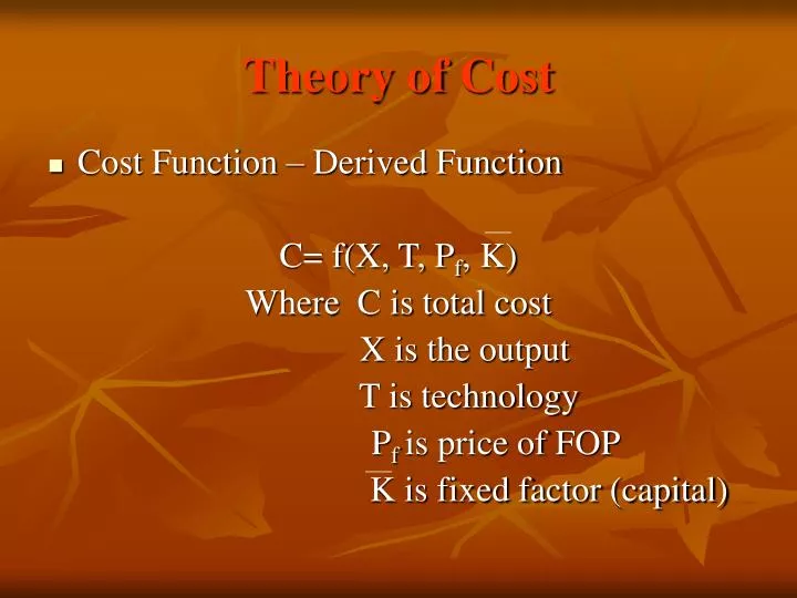
Theory of Cost. Cost Function – Derived Function C= f(X, T, P f , K) Where C is total cost X is the output T is technology P f is price of FOP K is fixed factor (capital). Cost Concepts.

E N D
Theory of Cost • Cost Function – Derived Function C= f(X, T, Pf, K) Where C is total cost X is the output T is technology Pf is price of FOP K is fixed factor (capital)
Cost Concepts • Opportunity Cost & Actual Concepts • Business Costs & Full Costs • Explicit & Implicit or Imputed Costs • Out-of-Pocket & Book Costs • Fixed & Variable Costs • Total, Average & Marginal Costs • Short-Run and Long-Run Costs • Incremental Costs and Sunk Costs • Historical & Replacement Costs • Private & Social Costs
Opportunity Cost & Actual Concepts • Opportunity cost refers to the expected returns from the second best use of resources which are foregone due to the scarcity of resources. • Actual cost are those which are actually incurred by the firm in the payment for labour, material , machinery, equipment etc.
Business cost and full cost • All the expenses which are incurred to carry out a business. The concept of business cost is similar to actual cost. • Full cost includes business cost, opportunity cost and normal profit. Normal profit is the necessary minimum earning which the firm must receive to remain in the present occupation.
Explicit & Implicit or Imputed Costs • Explicit costs = payments to non-owners of a firm for the supply of their resources (wages paid to labour, costs of electricity, the rental charges for plant usage, the cost of other raw materials used in the production process, etc.) • Implicit costs = the opportunity costs of using the resources already owned by the firm, where no payment is made to outsiders (use of the factory by giving up renting out for the same purpose, input of the owner / manager to give up the opportunity to earn a salary at another firm)
Out of Pocket and Book cost • The items of expenditure which involves cash payments or cash transfers are known as out of pocket cost. All the explicit cost like wages, rent, interest etc fall in this category. • Certain cost which do not involve cash payment but a provision is made while calculating profit and loss a/c are known as book cost. Eg. Unpaid interest on the owner’s own fund
Short run and Long run cost • Short run cost are the cost which vary with variation in the output, the size of the firm remaining the same. • Long run cost are the cost incurred on fixed assets like plant & machinery etc.
Historical and Replacement cost • Historical cost refers to the cost of the asset acquired in the past • Replacement cost refers to the outlay which has to be made for the replacement of old asset.
Incremental cost and sunk cost • Incremental cost refers to the total additional cost associated with the decision to expand the output. • Sunk cost are the cost that cannot be altered , increased or decreased by varying the rate of output. These are the cost that cannot be recovered. For eg. Amortization of past expenses like depreciation , expenditure on a highly specialized equipment designed to order for a plant that can neither be sold to any other firm nor can be used for any alternative purpose.
Private cost and social cost • Private cost refers to the cost of production incurred and provided for by the individual firm engaged in production of the commodity. It includes both explicit and implicit cost. • Social cost refers to the cost of producing the commodity to the society as the whole. It takes into consideration all those cost borne by the society directly or indirectly.
Traditional Theory – Short Run Cost TC = TFC + TVC • Total fixed cost: costs that do not vary with output and must be paid even if output is zero. These types of costs are beyond managerial control. Examples: Depreciation of machinery, rent, mortgage payments, interest payments on loans, and monthly connection fees for utilities. The level of total fixed costs is the same at all levels of output (even when output equals zero). • Total variable cost: costs that vary as output changes. If a firm uses more inputs to produce output, total variable costs will rise. These types of costs are within management control. Examples: labour costs, raw material costs, and running expenses such as fuel, ordinary repair & routine maintenance. Variable costs are equal to zero when no output is produced and increase with the level of output.
TC TVC TFC Fig. : Total Cost Curves Cost Output
Explanation for the total cost curve • Total fixed costs are the same at all levels of output, a graph of the total fixed cost curve is a horizontal line. • The total variable cost curve increases as output increases. Initially, it is expected to increase at a decreasing rate (since marginal productivity increases initially, the cost of additional units of output decline). As the level of output rises, however, variable costs are expected to increase at an increasing rate (as a result of the law of diminishing marginal returns).
TC, TVC, TFC • The table below contains a listing of a hypothetical set of total fixed cost and total variable cost schedules. As this table indicates, total fixed costs are the same at each possible level of output. Total variable costs are expected to rise as the level of output rises. • As the table below indicates, we can use the TFC and TVC schedules to determine the total cost schedule for this firm. Note that, at each level of output, TC = TFC + TVC.
AC = AFC + AVC • Average costs: costs per unit of output • Average fixed cost = TFC divided by quantity produced. • AFC = TFC / Q • as output rises AFC falls continuously (resembles a rectangular hyperbola) • Average variable cost = TVC divided by quantity produced • AVC = TVC / Q • usually average variable cost is U-shaped, with AVC falling initially and then rising as it becomes more costly to produce additional units of output. • Average total costs = AFC + AVC = TC/Q
ATC AVC AFC Fig. : Average costs Cost Output
Marginal Cost Marginal Cost (MC): Change in total costs due to a unit change in output. MC is the slope of TC curve. With an inverse S-shape of TC, MC curve will be U shape.
MC Fig.: Average and marginal costs Cost ATC Output
Relationship between MC & ATC • If the MC is less than the ATC, then the ATC must be falling. This follows from the fact that if you add a quantity to the average costs that is less than the average, the average must fall. • If the MC exceeds the ATC, the ATC must be rising. This follows from the fact that you are adding a quantity to the average costs that is greater than the average. Hence the average must rise. • It should also be noted that when MC cuts the ATC and the AVC at their minimum points.
MC AFC Fig .: Traditional Theory Cost Cost ATC AVC Output
Traditional Theory -Long run costs/Envelope Curve • The firm plans in the long run, when all inputs are variable • The LRAC is often called the firm’s planning curve. • The long run average cost (LRAC) is derived from short run cost curves. Each point of LRAC corresponds to a point on short run cost curve, which is tangent to LRAC.
Long-Run Average Costs • The LRAC is a curve that is tangent to the set of SRACs. When the LRAC curve falls the tangency points are to the left of the minimum points on the SRAC and when the LRAC curve is rising the tangency points are to the right of the minimum points of the SRAC curves. • With a great variety of plant sizes, the corresponding short-run average total cost curves trace a smooth LRAC curve.
Fig. :The LRAC or ‘the firm’s planning curve’ Cost SRATCl SRATCs SRATCm 40 30 Output 6 12 The plant size selected in the long-run depends on the expected level of production
LRAC is tangent to the set of SRACs Fig. : The LRAC with unlimited plant size Cost LRAC Output
Minimum efficient scale Fig. : Scale economies Cost Constant returns to scale Economies of scale Diseconomies of scale Output • LRAC varies from industry to industry • Usually economies dominate diseconomies
Economies of scale • (a) internal economies • (b) external economies Diseconomies of scale • (a) internal – managerial and labour inefficiency • (b) external
Reasons for Economies of Scale… • Increasing returns to scale • Specialization in the use of labor and capital • Economies in maintaining inventory • Discounts from bulk purchases • Lower cost of raising capital funds • Spreading promotional and R&D costs • Management efficiencies
Reasons for Diseconomies of Scale… • Decreasing returns to scale • Input market imperfections • Management coordination and control problems
Long Run Marginal Cost • LRMC is derived from SRMC, but does not envelope them. • LRMC is formed from points of intersections of SRMC curves with vertical lines drawn from point of tangency of corresponding SAC curve and LRAC curve. • At the minimum point we have SACB = SMCB = LAC = LMC
LMC SAC3 SMC3 SMC1 SAC2 LAC SAC1 SMC2
Break Even Analysis/Profit Contribution Analysis Linear Cost & Revenue Function
Break Even Analysis/Profit Contribution Analysis Non Linear Cost & Revenue Function
Modern Theory of Cost Need for Reserve Capacity • To meet seasonal & cyclical fluctuations in demand. • To give flexibility for repair of broken down machinery. • To increase output as demand increases. • To give flexibility for minor alterations of the product due to change in taste of customers. • Some reserve capacity on organizational & administrative level will also be required.
Difference b/w Reserve Capacity & Excess Capacity • Excess capacity arises from U-shaped costs by the traditional theory of the firm. While reserve capacity arises from the saucer shaped cost of modern theory of firm. • The traditional theory assumes that each plant is designed to produce optimally only single level of output. While the reserve capacity makes it possible to have constant SAVC within a certain range of output.
Difference b/w Reserve Capacity & Excess Capacity • The modern theory with change in output cost does not change while in traditional theory the cost also changes. • In figure the firm produces an output of X smaller than XM thus (XM-X )is the excess capacity which leads to increase in cost. The range of output X1X2 reflects the plant reserve capacity which does not leads to increase in cost.
AVC Difference b/w Excess & Reserve Capacity C C AVC Reserve Capacity 0 X XM X 0 X2 Excess Capacity X1