Random Vectors and Matrices

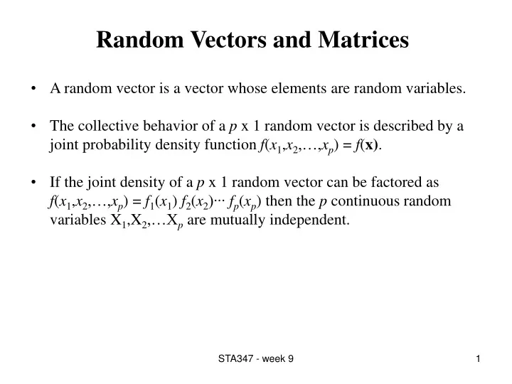
1. Random Vectors and Matrices • A random vector is a vector whose elements are random variables. • The collective behavior of a p x 1 random vector is described by a joint probability density function f(x1,x2,…,xp) = f(x). • If the joint density of a p x 1 random vector can be factored as f(x1,x2,…,xp) = f1(x1) f2(x2)∙∙∙ fp(xp) then the p continuous random variables X1,X2,…Xp are mutually independent. STA347 - week 9

2. Mean and Variance of Random Vector • The expected value of a random vector is a vector of the expected values of each of its elements. That is, the population mean vector is • The population variance-covariance matrix of a px1 random vector x is a p x p symmetric matrix where σij = Cov(Xi, Xj) = E(Xi– μi)(Xj– μj). • The population correlation matrix of a px1 random vector x is a p x p symmetric matrix ρ = (ρij) where STA347 - week 9

3. Properties of Mean Vector and Covariance Matrix STA347 - week 9

4. Functions of Random variables • In some case we would like to find the distribution of Y = h(X) when the distribution of X is known. • Discrete case • Examples 1. Let Y = aX + b , a≠ 0 2. Let STA347 - week 9

5. Continuous case – Examples 1. Suppose X ~ Uniform(0, 1). Let , then the cdf of Y can be found as follows The density of Y is then given by 2. Let X have the exponential distribution with parameter λ. Find the density for 3. Suppose X is a random variable with density Check if this is a valid density and find the density of . STA347 - week 9

6. Theorem • If X is a continuous random variable with density fX(x) and h is strictly increasing and differentiable function form RR then Y = h(X) has density for . • Proof: STA347 - week 9

7. Theorem • If X is a continuous random variable with density fX(x) and h is strictly decreasing and differentiable function form RR then Y = h(X) has density for . • Proof: STA347 - week 9

8. Summary • If Y = h(X) and h is monotone then • Example X has a density Let . Compute the density of Y. STA347 - week 9

9. Change-of-Variable for Joint Distributions • Theorem Let X and Y be jointly continuous random variables with joint density function fX,Y(x,y) and let DXY = {(x,y): fX,Y(x,y) >0}. If the mapping T given by T(x,y) = (u(x,y),v(x,y)) maps DXY onto DUV. Then U, V are jointly continuous random variable with joint density function given by where J(u,v) is the Jacobian of T-1 given by assuming derivatives exists and are continuous at all points in DUV . STA347 - week 9

10. Example • Let X, Y have joint density function given by Find the density function of STA347 - week 9

11. Example • Show that the integral over the Standard Normal distribution is 1. STA347 - week 9

12. Example • A device containing two key components fails when and only when both components fail. The lifetime, T1 and T2, of these components are independent with a common density function given by • The cost, X, of operating the device until failure is 2T1 + T2. Find the density function of X. STA347 - week 9

13. Convolution • Suppose X, Y jointly distributed random variables. We want to find the probability / density function of Z=X+Y. • Discrete case X, Y have joint probability function pX,Y(x,y). Z = z whenever X = x and Y = z – x. So the probability that Z = z is the sum over all x of these joint probabilities. That is • If X, Y independent then This is known as the convolution of pX(x) and pY(y). STA347 - week 9

14. Example • Suppose X~ Poisson(λ1) independent of Y~ Poisson(λ2). Find the distribution of X+Y. STA347 - week 9

15. Convolution - Continuous case • Suppose X, Y random variables with joint density function fX,Y(x,y). We want to find the density function of Z=X+Y. Can find distribution function of Z and differentiate. How? The Cdf of Z can be found as follows: If is continuous at z then the density function of Z is given by • If X, Y independent then This is known as the convolution of fX(x) and fY(y).

16. Example • X, Y independent each having Exponential distribution with mean 1/λ. Find the density for W=X+Y. STA347 - week 9

17. Order Statistics • The order statistics of a set of random variables X1, X2,…, Xn are the same random variables arranged in increasing order. • Denote by X(1) = smallest of X1, X2,…, Xn X(2) = 2nd smallest of X1, X2,…, Xn X(n) = largest of X1, X2,…, Xn • Note, even if Xi’s are independent, X(i)’s can not be independent since X(1) ≤ X(2) ≤… ≤ X(n) • Distribution of Xi’s and X(i)’s are NOT the same. STA347 - week 9

18. Distribution of the Largest order statistic X(n) • Suppose X1, X2,…, Xn are i.i.d random variables with common distribution function FX(x) and common density function fX(x). • The CDF of the largest order statistic, X(n), is given by • The density function of X(n) is then STA347 - week 9

19. Example • Suppose X1, X2,…, Xn are i.i.d Uniform(0,1) random variables. Find the density function of X(n). STA347 - week 9

20. Distribution of the Smallest order statistic X(1) • Suppose X1, X2,…, Xn are i.i.d random variables with common distribution function FX(x) and common density function fX(x). • The CDF of the smallest order statistic X(1) is given by • The density function of X(1) is then STA347 - week 9

21. Example • Suppose X1, X2,…, Xn are i.i.d Uniform(0,1) random variables. Find the density function of X(1). STA347 - week 9

22. Distribution of the kth order statistic X(k) • Suppose X1, X2,…, Xn are i.i.d random variables with common distribution function FX(x) and common density function fX(x). • The density function of X(k) is STA347 - week 9

23. Example • Suppose X1, X2,…, Xn are i.i.d Uniform(0,1) random variables. Find the density function of X(k). STA347 - week 9

24. Computer Simulations - Introduction Modern high-speed computers can be used to perform simulation studies. Computer simulation methods are commonly used in statistical applications; sometimes they replace theory, e.g., bootstrap methods. Computer simulations are becoming more and more common in many applications such as quality control, marketing, scientific research etc. STA347 - week 9 24

25. Applications of Computer Simulations Our main focus is on probabilistic simulations. Examples of applications of such simulations include: Simulate probabilities and random variables numerically. Approximate quantities that are too difficult to compute mathematically. Random selection of a sample from a very large data sets. Encrypt data or generate passwords. Generate potential solutions for difficult problems. STA347 - week 9 25

26. Steps in Probabilistic Simulations In most applications, the first step is to specify a certain probability distribution. Once such distribution is specified, it will be desired to generate one or more random variables having that distribution. The build-in computer device that generates random numbers is calledpseudorandom number generator. It is a device for generating a sequence U1, U2, … of random values that are approximately independent and have approximately uniform distribution of the unit interval [0,1]. STA347 - week 9 26

27. Simulating Discrete Distributions - Example Suppose we wish to generate X ~ Bernoulli(p), where 0 < p < 1. We start by generating U ~ Uniform[0, 1] and then set: Then clearly X takes two values, 0 and 1. Further, Therefore, we have that X ~ Bernoulli(p). This can be generalized to generate Y ~ Binomial(n, p) by generating U1, U2, … Un. Setting Xi as above and let Y = X1 + ∙∙∙ + Xn. STA347 - week 9 27

28. Simulating Discrete Distributions In general, suppose we wish to generate a random variable with probability mass function p. Let, x1 < x2 < x3 < ∙∙∙ be all the values for which p(xi) > 0. Let U ~ Uniform[0, 1]. Define Y by: Theorem 1:Y is a discrete random variable, having probability mass function p. Proof: STA347 - week 9 28

29. Simulating Continuous Distributions - Example Suppose we wish to generate X ~ Uniform[a, b]. We start by generating U ~ Uniform[0, 1] and then set: Using one-dimensional change of variable theorem we can easily show that X ~ Uniform[a, b]. STA347 - week 9 29

30. Simulating Continuous Distributions In general, simulating continuous distribution is not an easy task. However, for certain continuous distributions it is not difficult. The general method for simulating continuous distribution makes use of the inverse cumulative distribution function. The inverse cdf of a random variable X with cumulative distribution function F is defined by: for 0 < t < 1. STA347 - week 9 30

31. Inversion Method for Generating RV Let F be any cumulative distribution function, and let U ~ Uniform[0, 1]. Define a random variable Y by: Theorem 2:Y has cumulative distribution function given by F. That is, Proof: STA347 - week 9 31

32. Important Notes The theorem above is valid for any cumulative distribution function whether it corresponds to a continuous distribution, a discrete distribution or a mixture of the two. The inversion method for generating random variables described above can be used whenever the distribution function is not too complicated and has a close form. For distributions that are too complicated to sample using the inversion method and for which there is no simple trick , it may still be possible to generate samples using Markov chain methods. STA347 - week 9 32

33. Example – Exponential Distribution • Suppose X ~ Exponential(λ). The probability density function of X is: • The cdf of X is: • Setting and solving for x we get… • Therefore, by theorem 2 above, where U ~ Uniform[0, 1], has an Exponential(λ) distribution. STA347 - week 9 33

34. Example – Standard Normal Distribution • Suppose X ~ Normal(0,1). The cdf of X is denoted by Ф(x). It is given by: • Then, if U ~ Uniform[0, 1], by theorem 2 above has a N(0,1) distribution. • However, since both Ф and Ф-1 don’t have a close form, i.e., it is difficult to compute them, the inversion method for generating RV is not practical. STA347 - week 9 34