V18 Stochastic simulations of cellular signalling

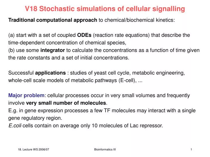
1. V18 Stochastic simulations of cellular signalling Traditional computational approach to chemical/biochemical kinetics: (a) start with a set of coupled ODEs (reaction rate equations) that describe the time-dependent concentration of chemical species, (b) use some integrator to calculate the concentrations as a function of time given the rate constants and a set of initial concentrations. Successful applications : studies of yeast cell cycle, metabolic engineering, whole-cell scale models of metabolic pathways (E-cell), ... Major problem: cellular processes occur in very small volumes and frequently involve very small number of molecules. E.g. in gene expression processes a few TF molecules may interact with a single gene regulatory region. E.coli cells contain on average only 10 molecules of Lac repressor. Bioinformatics III

2. Include stochastic effects (Consequence1)  modeling of reactions as continuous fluxes of matter is no longer correct. (Consequence2) Significant stochastic fluctuations occur. To study the stochastic effects in biochemical reactions stochastic formulations of chemical kinetics and Monte Carlo computer simulations have been used. Daniel Gillespie (J Comput Phys 22, 403 (1976); J Chem Phys 81, 2340 (1977)) introduced the exact Dynamic Monte Carlo (DMC) method that connects the traditional chemical kinetics and stochastic approaches. Assuming that the system is well mixed, the rate constants appearing in these two methods are related. Bioinformatics III

3. Dynamic Monte Carlo In the usual implementation of DMC for kinetic simulations, each reaction is considered as an event and each event has an associated probability of occurring. The probability P(Ei) that a certain chemical reaction Ei takes place in a given time interval t is proportional to an effective rate constant k and to the number of chemical species that can take part in that event. E.g. the probability of the first-order reaction X  Y + Z would be k1Nx with Nx :number of species X, and k1 : rate constant of the reaction Similarly, the probability of the reverse second-order reaction Y + Z  X would be k2NYNZ. Resat et al., J.Phys.Chem. B 105, 11026 (2001) Bioinformatics III

4. Dynamic Monte Carlo As the method is a probabilistic approach based on „events“, „reactions“ included in the DMC simulations do not have to be solely chemical reactions. Any process that can be associated with a probability can be included as an event in the DMC simulations. E.g. a substrate attaching to a solid surface can initiate a series of chemical reactions. One can split the modelling into the physical events of substrate arrival, of attaching the substrate, followed by the chemical reaction steps. Resat et al., J.Phys.Chem. B 105, 11026 (2001) Bioinformatics III

5. Basic outline of the direct method of Gillespie (Step i) generate a list of the components/species and define the initial distribution at time t = 0. (Step ii) generate a list of possible events Ei (chemical reactions as well as physical processes). (Step iii) using the current component/species distribution, prepare a probability table P(Ei) of all the events that can take place. Compute the total probability P(Ei) : probability of event Ei. (Step iv) Pick two random numbers r1 and r2  [0...1] to decide which event E will occur next and the amount of time  by which E occurs later since the most recent event. Resat et al., J.Phys.Chem. B 105, 11026 (2001) Bioinformatics III

6. Basic outline of the direct method of Gillespie Using the random number r1 and the probability table, the event E is determined by finding the event that satisfies the relation The second random number r2 is used to obtain the amount of time  between the reactions As the total probability of the events changes in time, the time step between occurring steps varies. Steps (iii) and (iv) are repeated at each step of the simulation. The necessary number of runs depends on the inherent noise of the system and on the desired statistical accuracy. Resat et al., J.Phys.Chem. B 105, 11026 (2001) Bioinformatics III

7. Weighted Sampling In the commonly used MC algorithm, the Markov chain is generated using transition probabilities (i  j) that are based on the physical probability distribution: The ensemble average  of any physical quantity  is obtained by taking the arithmetic average of all the n simulation runs. The individual averages i could e.g. be time-averages over the simulation run. This choice disfavors the transitions with low probabilities. If the system characteristics depend on the events that happen less frequently, then the common implementation of MC requires extremely lengthy simulations to acquire enough statistical sampling. Resat et al., J.Phys.Chem. B 105, 11026 (2001) Bioinformatics III

8. Weighted Sampling This statistical sampling problem can be avoided if the probability distribution is multiplied with a weight function that adjusts the sampling probability distribution such that the low probability parts of the sampling space are visited more often. In the case of weighted sampling, the Markov chain is generated by using the modified probability distribution function where Y is the biasing weight function. Since the probability of the transition i  j is weighted with Y(i  j), calculation of the ensemble average of a physical quantity  is obtained by computing the average of  / Y. Division of  by Y effectively corrects for the bias introduced in the sampling probability distribution. Resat et al., J.Phys.Chem. B 105, 11026 (2001) Bioinformatics III

9. Probability-Weighted DMC Probability-weighted DMC incorporates weighted sampling into DMC. Steps (iii) and (iv) of the DMC algorithm are replaced by (Step iii‘) Using the current component/species distribution, prepare a probability table of all the events Ei that can take place, (Step iv‘) define the weight factor scale and compute the inverse probability weight table for all events. Note that the stochastic simulations mentioned here use discrete numbers of molecules, i.e. the species are produced and consumed as whole integer units. Therefore, the weight table w(E ) must contain only integer values. Resat et al., J.Phys.Chem. B 105, 11026 (2001) Bioinformatics III

10. Probability-Weighted DMC (Step v‘) Prepare the weighted probability table (Step vi‘) Compute the total probability by summing the weighted probabilities of all individual events (Step vii‘) Pick two random numbers r1,r2 [0...1]. Determine which event E occurs next as before using r1. (Step viii‘) Propagate the time as before using r2. The speed-up achieved by the PW-DMC algorithm stems from the fact that the reactions with large probabilities are allowed to occur in „bundles“. Resat et al., J.Phys.Chem. B 105, 11026 (2001) Bioinformatics III

11. Comparison of DMC and PW-DMC DMC is essentially a method to solve the master equation that rules how the probabilities of the configurations are related to each other W : transition probability of going from configuration  to  P : probability of configuration . Using the master equation, the statistical average X of the rate of change of the property X can be expressed as: In PW-DMC, this relation is rearranged using the weight factor w as PW-DMC leaves the ensemble averages unchanged. However, the fluctuations increase with w. Resat et al., J.Phys.Chem. B 105, 11026 (2001) Bioinformatics III

12. Integrated Model of Epidermal Growth Factor Receptor Trafficking and Signal Transduction The EGF receptor can be activated by the binding of any one of a number of different ligands. Each ligand stimulates a somewhat different spectrum of biological responses. The effect of different ligands on EGFR activity is quite similar at a biochemical level  the mechanisms responsible for their differential effect on cellular responses are unkown. After binding of any of its ligands, EGFR is rapidly internalized by endocytosis. Resat et al. Biophys Journal 85, 730 (2003) Bioinformatics III

13. Computational modelling of EGF receptor system (1) trafficking and ligand-induced endocytosis (2) signaling through Ras or MAP kinases This work combines both aspects into a single model. Most approaches to building computational kinetic models have severe drawbacks when representing spatially heterogenous processes on a cellular scale. Review: In the traditional approach, we - formulate set of coupled ODEs (reaction rate equations) for the time-dependent concentration of chemical species - use integrator to propagate the concentrations as a function of time given the rate constants and a set of initial concentrations. Resat et al. Biophys Journal 85, 730 (2003) Bioinformatics III

14. Multiple time scale problem In Dynamic Monte Carlo, reactions are considered events that occur with certain probabilities over set intervals of time. The event probabilities depend on the rate constant of the reaction and on the number of molecules participating in the reaction. In many interesting natural problems, the time scales of the events are spread over a large spectrum. Therefore it is very inefficient to treat all processes at the time scale of the fastest individual reaction. In the EGFR signaling network, - receptor phosphorylation after ligand binding occurs almost instantaneously - vesicle formation or sorting to lysosomes requires many minutes. Resat et al. Biophys Journal 85, 730 (2003) Bioinformatics III

15. Solution to multiple time scale problem Computing millions and billions non-correlated random numbers can become a time-consuming process. Resat et al. (2001) introduced Probability-Weighted DMC to speed-up the simulation by factor 20 – 100. Different processes are only tested at variant times depending on their probabilities = very unlikely processes compute MC decision very infrequently. Resat et al. Biophys Journal 85, 730 (2003) Bioinformatics III

16. Signal transduction model of EGF receptor signaling pathway Resat et al. Biophys Journal 85, 730 (2003) Bioinformatics III

17. Species in the EGF receptor signaling model Resat et al. Biophys Journal 85, 730 (2003) Bioinformatics III

18. Receptor and ligand group definitions Resat et al. Biophys Journal 85, 730 (2003) Bioinformatics III

19. Early endosome inclusion coefficients These are adjusted to yield the experimentally determined rates of ligand-free and ligand-bound receptor internalization. Resat et al. Biophys Journal 85, 730 (2003) Bioinformatics III

20. Time course of phosphorylated EGF receptors (a) Total number of phosphorylated EGF receptors in the cell. Curves represent the number of activated receptors when the cell is stimulated with different ligand doses at the beginning. The y axis represents the number of receptors in thousands. (b ) Ratio of the number of phosphorylated receptors that are internalized to that of the phosphorylated surface receptors. (c) Ratio of the number of internalized receptors to the number of surface receptors. Curves are colored as: [L] = 0.2 (magenta), 1 (blue), 2 (green), and 20 (red) nM. Resat et al. Biophys Journal 85, 730 (2003) Bioinformatics III

21. Distribution of the receptors among cellular compartments Resat et al. Biophys Journal 85, 730 (2003) Bioinformatics III

22. Stimulation of EGFR signaling pathway by different ligands Comparison of the results when the EGFR signaling pathway is stimulated with its ligands EGF (red) and TGF- (green). (a ) Total number of receptors in the cell as a function of time after 20 nM ligand is added to the system. Red diamond (EGF) and green square (TGF-) points show the experimental results. (b) Distribution of the receptors between intravesicular compartments and the cell membrane. (c) Distribution of the phosphorylated receptors between intravesicular compartments and the cell membrane. In the figures, y axes represent the number of receptors in thousands. Resat et al. Biophys Journal 85, 730 (2003) Bioinformatics III

23. Ratio of internal/surface receptors The ratio of the In/Sur ratios when the EGFR signaling pathway is stimulated with its ligands EGF and TGF- at 20 nM ligand concentration. Comparison of computational (solid lines) and experimental (points) results. Ratio of the ratios for the phosphorylated (i.e., activated) (blue), and total (phosphorylated + unphosphorylated) number (magenta) of receptors. Resat et al. Biophys Journal 85, 730 (2003) Bioinformatics III

24. Summary Large-scale simulations of the kinetics of biological signaling networks are becoming feasible. Here, the model consisted of hundreds of distinct compartments and ca. 13.000 reactions/events that occur on a wide spatial-temporal range. The exact Dynamic Monte Carlo algorithm of Gillespie (1976/1977) was a breakthrough for simulations of stochastic systems. Problem: simulations can become very time-consuming. In particular if the processes occur on different time scales. Methods like the probability-weighted DMC are promising tools for studying complex cellular systems using molecular quanta. Many other variants of DMC have and are being development. Bioinformatics III

25. Bacterial Photosynthesis 101 ATPase Photons Reaction Center chemical energy e––H+–pairs light energy outside inside Light Harvesting Complexes cytochrome bc1complex ubiquinon cytochrome c2 electronic excitation H+ gradient; transmembrane potential electron carriers Bioinformatics III

26. Modelling as metabolic network Chemical reactions involved: Bioinformatics III

27. 2 cycles: electrons protons Photosynthesis – cycle view The conversion chain: stoichiometries must match turnovers! H+ gradient, transmembrane voltage electronic excitation chemical energy e––H+–pairs light energy outside inside Bioinformatics III

28. LH2: 8 αβ dimers LH1: 16 αβ dimers downhill transport of excitons LH2  LH1 RC B800, B850, Car. LH1 / LH2 / RC — a la textbook Collecting photons Bioinformatics III Hu et al, 1998

29. Q-cycle: Berry, etal, 2004 X-ray structures known always forms a dimer 2H+ per 1e– The Cytochrome bc1complex the "proton pump" Bioinformatics III

30. per turn: 10–14 H+ 3 ATP 1 ATP ≙ 4 H+ Capaldi, Aggeler, 2002 The FoF1-ATP synthase I at the end of the chain: producing ATP from the H+ gradient Bioinformatics III

31. The electron carriers Cytochrome c: electrons from bc1 to RC • heme in a hydrophilic protein shell • 3.3 nm diameter Ubiquinon UQ10: carries electron–proton pairs from RC to bc1 • hydrophobic tail • long (2.4 nm) isoprenoid tail taken from Stryer Bioinformatics III

32. Bahatyrova et al., 2004 no bc1 found! 100 nm 100 nm LH1 200 nm * bc1? RC 50 nm Tubular membranes – photosynthetic vesicleswhere are the bc1 complexes and the ATPase? Jungas et al., 1999 Bioinformatics III

33. Chromatophore vesicle: typical form in Rh. sphaeroides Lipid vesicles 30–60 nm diameter H+ and cyt c inside average chromatophore vesicle, 45 nm Ø: surface 6300 nm² Vesicles are really small! Bioinformatics III

34. dE/dλ [arb.] Wavelength [nm] γ s kW Bchl capture rate: 0.1 Photon capture rate of LHC’s relative absorption spectrum of LH1/RC and LH2 sun's spectrum at ground (total: 1 kW/m²) multiply Gerthsen, 1985 Cogdell etal, 2003 + Bchl extinction coeff. normalization (Bchl = 2.3 Å2) Franke, Amesz, 1995 typical growth condition: 18 W/m² Feniouk et al, 2002 LH1: 16 * 3 Bchl  14 γ/s LH2: 10 * 3 Bchl  10 γ/s Bioinformatics III

35. LH1 / LH2 / RC — native electron micrograph and density map Siebert etal, 2004 125 * 195 Ų, γ = 106° Chromatophore vesicle, 45 nm Ø: surface 6300 nm² Bioinformatics III

36. Photon processing rate at the RC Which process limits the RCs turnover? Unbinding of the quinol  25 ms Milano et al. 2003 + binding, charge transfer ≈ 50 ms per quinol (estimate) with 2e- H+ pairs per quinol 40–50 γ/s per RC  22 QH2/s 1 RC can serve 1 LH1 + 3 LH2 = 44 γ/s LH12+ 6 LH2 ≙ 456 nm²  11 LH1 dimers including 22 RCs on one vesicle  480 Q/s can be loaded @ 18 W/m² per vesicle Bioinformatics III

37. limited throughput of the ATPase  1 ATP ≙ 4 H+ "binding" 1 ATPase per vesicle "Arrhenius" Gräber et al, 1991, 1999 Feniouk et al, 2002 The F1F0-ATP synthase "…mushroom like structures observed in AFM images…"  ATPase is "visible" per turn: 10–14 H+per 3 ATP Bioinformatics III

38. How much bc1? measured enzymatic activity per bc1 dimer: 84 cyt c are reduced / s Xiao et al. 2000 in out  1 dimer "pumps" 168 H+ / s  1 dimer can process 42 QH₂ / s 400 H+ / s per ATPase x5 !!!  proton generation by 2.4 bc1 dimers per vesicle enough to drive 1 ATPase  11 bc1 dimers per vesicle can be loaded by RCs safety first! number of bc1complexes should be limited by how many protons can be pumped out by ATPase Bioinformatics III

39. Diffusion is not limiting bc1 Placement — Diffusional limits? Roundtrip times maximal capacity of the carriers: T = TRC + Tbc1 + TDîff Cytochrome c₂: TRC ≈ 1 ms Tbc1 ≈ 12 ms TDiff ≈ 3 μs Tround-trip = 13 ms  ≤ 3 cyt c per vesicle sufficient to carry e-‘s available: 22 cyt c per vesicle Quinol: TRC ≈ 50 ms Tbc1 ≈ 23 ms TDiff ≈ 1 ms Tround-trip = 75 ms  ≤ 7 Q per vesicle sufficient to carry e-’s.  poses no constraints for the position of bc1 available: 100 Q per vesicle Bioinformatics III

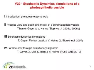
40. Proposed setup of a chromatophore vesicle At the „poles“ green/red: the ATPase light blue: the bc1 complexes Increased proton density close to the ATPase. favors close placing ATPase and bc1 complexes. yellow arrows: diffusion of the protons out of the vesicle via the ATPase and to the RCs and bc1s. blue: small LH2 rings (blue) blue/red: Z-shaped LH1/RC dimers form a linear array around the “equator” of the vesicle, determining the vesicle’s diameter by their intrinsic curvature. Geyer, Helms, Biophys. J. (2006) 91, 921 Bioinformatics III

41. reconstituted LH1 dimers in planar lipid membranes Upper panel: drawn after the AFM images of Scheuring et al (4) of LH1 dimers reconstituted into planar lipid membranes. The Z-shaped dimers are seen from their cytoplasmic side. The average height of the membrane is indicated in the upper panel by the grey level of the background. Scheuring et al measured the distances between the minima of the AFM height scan to be 38.5 nm and the distance be tween the lowest and the highest parts to be 3.8 nm. Lower panel: interpretation how alternatingly oriented LH1 dimers may explain the observed height scan indicated by the dashed lines. These values are nicely reproduced by the proposed arrangement of the LH1 dimers, when one assumes that they are stiff enough to retain the bending angle of 26 that they would have on a spherical vesicle of 45 nm diameter and taking into account the length of a single LH1 dimer of about 19.5 nm. Bioinformatics III

42. Photosynthesis: textbook view Bioinformatics III

43. Viewing the photosynthetic apparatus as a conversion chain Thick arrows : path through which the photon energy is converted into chemical energy stored in ATP via the intermediate stages (rounded rectangles). Each conversion step takes place in parallely working proteins. Their number N times the conversion rate of a single protein R determines the total throughput of this step.  : incoming photons collected in the LHCs E : excitons in the LHCs and in the RC e−H+ electron–proton pairs stored on the quinols e− for the electrons on the cytochrome c2 pH : transmembrane proton gradient H+ : protons outside of the vesicle (broken outine of the respective reservoir). Bioinformatics III

44. Modelling of internal processes at reaction center All individual reactions with their individual rates k together determine the overall conversion rate RRC of a single RC. Thick arrows : flow of the energy from the excitons through the cyclic charge state changes of the special pair Bchl (P) of the RC. Rounded rectangles : reservoirs Bioinformatics III

45. Parameters Bioinformatics III

46. Stochastic dynamics simulations II Production runs fixed set of parameters integrate rate equations with: - Gillespie algorithm (associations) - Timer algorithm (reactions); 1 random number determines when reaction occurs Bioinformatics III

47. example: binding and e- transfer at reaction center Bioinformatics III

48. Stochastic simulations of a complete vesicle Model vesicle: 12 LH1/RC-monomers 1-6 bc1complexes 1 ATPase 120 quinones 20 cytochrome c2 integration time step: 10 s simulating 1 minute real time requires 1.5 minute on one opteron 2.4 GHz proc Bioinformatics III

49. simulate increase of light intensity during 1 minute, light intensity was slowly increased from 0 to 10 W/m2 (quasi steady state)  there are two regimes - one limited by available light - one limited by bc1 throughput low light intensity: linear increase of ATP production with light intensity high light intensity: saturation is reached the later the higher the number of bc1 complexes Geyer, Lauck, Helms, J. Biotech (to be accepted) Bioinformatics III

50. oxidation state of cytochrome c2 pool low light intensity: all 20 cytochrome c2 are reduced by bc1 high light intensity RCs are faster than bc1, c2s wait for electrons Bioinformatics III