Download
1 / 17
170 likes | 375 Views
A model for comparing means. (Session 12). Learning Objectives. At the end of this session, you will be able to understand and interpret the components of a linear model for comparing means make comparisons from an examination of the parameter estimates via t-tests

E N D
A model for comparing means (Session 12)
Learning Objectives At the end of this session, you will be able to • understand and interpret the components of a linear model for comparing means • make comparisons from an examination of the parameter estimates via t-tests • describe assumptions associated with a linear model for two categorical factors • conduct a residual analysis to check model assumptions
A model for the paddy data Consider again the objective of comparing paddy yields across the 3 varieties. A linear model for this data takes the form: yij =0+ gi + ij ,i = 1, 2, 3 Here 0 represents a constant, and the gi represent the variety effect. Estimates of 0 and gi can be obtained with appropriate software.
A model for the paddy data Graph showing the model: yij =0+ gi + ij,i = 1, 2, 3 Mean value for old improved variety Grand mean=4.06 New imp Old imp Traditional
Model estimates and anova What do these results tell us?
Graph showing model again yij =0+ gi + ij,i = 1, 2, 3 Mean for variety i = constant + gi = 5.96 + gi, where g1 = 0, g2 = -1.416, g3 = -2.96 Mean value of new improved variety at 5.96 New imp Traditional Old imp
Relating estimates to means Thus comparison with the “first” level becomes easy – and t-tests (slide 5) can be interpreted as comparisons with this level.
Other comparisons How do we compare old with traditional? First note (using parameter estimates) that Old-Trad = (Old-New)-(Trad-New) = g2-g3 = - 1.416 - (-2.960) = 1.544 This is the same as the difference in means between the two varieties (see below).
Finding the standard error But how can the std. error be found? For this, the variance-covariance matrix between parameter estimates is needed, (see below) followed by some computations. Variances are the diagonal elements, co-variances are the off-diagonal elements
Computing the standard error Need Var(g2-g3) = Var(g2)+Var(g3)-2covar(g2,g3) = 0.1335 + 0.1369 – 2(0.1081) = 0.0542 Hence, std error(g2-g3) = 0.0542 = 0.2328 So t-test for the comparison will be t = 1.544 / 0.2328 = 6.63, which is clearly a highly significant result. So clear evidence of a difference between old improved and traditional varieties.
Model Assumptions Anova model with one categorical factors is: yij =0+ gi + ij As in linear regression, it is assumed that this model is linear. Additionally, the i are assumed to be • independent, with • zero mean and constant variance 2, • and be normally distributed. Note: As before, values predicted for yij are called fitted values.
Checking Model Assumptions Model assumptions are checked in exactly the same way as for regression analysis. A residual analysis is done, looking at plots of residuals in various ways. Such procedures are the same when modelling any quantitative response using a model linear in its unknown parameters. We give below a residual analysis for the model fitted above.
Histogram to check normality Histogram of standardised residuals after fitting a model of yield on variety.
A normal probability plot… Another check on the normality assumption Do you think the points follow a straight line?
Std. residuals versus fitted values Checking assumption of variance homogeneity, and identification of outliers: Is this plot satisfactory? The straight vertical lines appear because variety has just 3 distinct values.
Conclusions • There was little indication to doubt any of the assumptions associated with the model. • There was clear evidence that the varieties differed in terms of the corresponding mean paddy yields. • The new improved variety gave highest production, showing an increase of 1.42 tonnes/ha with confidence interval (0.67, 2.16) over the old improved variety. • Least production was with the traditional variety.
Practical work follows to ensure learning objectives are achieved…