Triangulation of Monotone Polygon

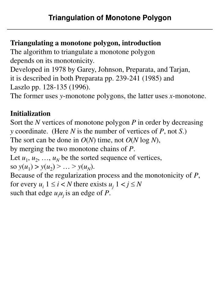
1. Triangulation of Monotone Polygon Triangulating a monotone polygon, introduction The algorithm to triangulate a monotone polygon depends on its monotonicity. Developed in 1978 by Garey, Johnson, Preparata, and Tarjan, it is described in both Preparata pp. 239-241 (1985) and Laszlo pp. 128-135 (1996). The former uses y-monotone polygons, the latter uses x-monotone. Initialization Sort the N vertices of monotone polygon P in order by decreasing y coordinate. (Here N is the number of vertices of P, not S.) The sort can be done in O(N) time, not O(N log N), by merging the two monotone chains of P. Let u1, u2, …, uN be the sorted sequence of vertices, so y(u1) > y(u2) > … > y(uN). Because of the regularization process and the monotonicity of P, for every ui 1 i < N there exists uj 1 < jN such that edge uiujis an edge of P.

2. ProximityConstrained triangulation Description of the processing The algorithm processes one vertex at a time in order of decreasing y coordinate, creating diagonals of polygon P. Each diagonal bounds a triangle, and leaves a polygon with one less side still to be triangulated. Stack The algorithm uses a stack to store vertices that have been visited but not yet connected with a diagonal. The stack content is v1, v2, …, vi, where v1 is the bottom and vi the top of the stack. At any time during the execution, there are two invariants: 1. The vertices v1, v2, …, vi on the stack from a chain on the boundary of P, where y(v1) > y(v2) > … > y(vi). 2. If i 3, angle vjvj+1vj+2 for 1 ji - 2.

3. ProximityConstrained triangulation Algorithm By “adjacent” we mean connected by an edge in P. Recall that v1 is the bottom of the stack, vi is the top. 1. Push u1 and u2 on the stack. 2. j = 3 /* j is index of current vertex */ 3. u = uj 4. Case (i): u is adjacent to v1 but not vi. add diagonals uv2, uv3, …, uvi. pop vi, vi-1, …, v1 from stack. push vi, u on stack. Case (ii): u is adjacent to vi but not v1. while i > 1 and angle uvivi-1 <  add diagonal uvi-1 pop vi from stack endwhile push u Case (iii): u adjacent to both v1 and vi. add diagonals uv2, uv3, …, uvi-1. exit 5. j = j + 1 Go to step 3.

4. v1 v2 v3 v4 = vi top of stack u ProximityConstrained triangulation Algorithm cases Case (i): u is adjacent to v1 but not vi. v1 v2 v3 v4 = vi top of stack u Case (ii): u is adjacent to vi but not v1. v1 v2 v3 v4 v5 = vi top of stack u Case (iii): u adjacent to both v1 and vi.

5. v1 v1 v2 v2 v3 u u 2, Case (ii) 1, initial v1 v2 v3 v4 v1 u v2 u 3, Case (ii) 4, Case (i) ProximityConstrained triangulation Example, 1

6. v1 v1 v2 v2 u v3 u 5, Case (ii) 6, Case (ii) v1 v2 v3 v4 u 7, Case (ii) ProximityConstrained triangulation Example, 2 v1 v2 v3 8, Case (ii) u

7. ProximityConstrained triangulation Example, 3 9, Case (iii) 10, final

8. ProximityConstrained triangulation Proof of correctness The correctness of the algorithm depends on the fact that all the added diagonals lie inside the polygon P. For details, see Preparata pp. 240-241, or Laszlo pp. 134-135. Analysis of triangulating a monotone polygon The initial sort (merge) requires O(N) time. Each of the N vertices is visited and placed on the stack exactly once, except when the while fails in case (ii). This happens at most once per vertex, so that time can be charged to the current vertex.  The algorithm requires O(N) time to triangulate a monotone polygon, where N is the number of vertices of the polygon.

9. ProximityConstrained triangulation S, E (1) Inscribe S in minimum enclosing axis parallel rectangle. O(N) PSLG rect(S), S, E (2) Regularize rect(S), S, E. O(N log N) Each region within regularized rect(S), S, E is a monotone polygon. Regularized rect(S), S, E (3) Decompose regularized rect(S), S, E into monotone polygons. O(N) Monotone polygon (4) Triangulate monotone polygons. O(N) Triangulation of rect(S) Overall comments O(N log N) regularization dominates time. O(N) for triangulating all monotone polygons (here N is the number of vertices in S and rect(S). We know TRIANGULATION has lower bound in (N log N).  This algorithm is optimal, (N log N).

10. ProximityTriangulating a simple polygon Definitions In a simple polygon, edges intersect only at vertices, and non-adjacent edges do not intersect. Three consecutive vertices a, b, c of a polygon form an ear of the polygon if segment ac is a diagonal; b is the ear tip. Meister’s Two Ears Theorem. Every polygon with N 4 vertices has at least two nonoverlapping ears.

11. ProximityTriangulating a simple polygon Example, simple polygon with ears c b ear a

12. ProximityTriangulating a simple polygon Triangulation by otectomy See O’Rourke, pp. 39-46. Let P be a simple polygon, with vertices {p1, p2, …, pN}. 1. if N > 3 2. for each potential ear diagonal pipi+2 3. if pipi+2 is a diagonal 4. add diagonal pipi+2 5. recurse on P - {pi+1} 6. endif 7. endfor 8. endif Analysis Step 2 is O(N), search around P. Step 3 is a test for diagonal by checking for intersections, O(N). Step 5 can occur at most O(N) times. Overall time required is O(N3).

13. ProximityTriangulating a simple polygon Example p12 p5 7 p11 2 8 p10 10 p13 9 p7 p15 3 p6 11 p9 p14 p8 12 13 p16 4 p4 14 5 p17 1 6 15 p2 p18 p3 p1 Numbers indicate sequence in which diagonals were added.