Download
1 / 24
240 likes | 415 Views
VIC (Variable Infiltration Capacity) model recent developments and modifications. Dennis P Lettenmaier Civil and Environmental Engineering, University of Washington. EU-WATCH Project symposium April 10, 2009. Outline. General overview of the VIC model Multi-layer Snowpack

E N D
VIC (Variable Infiltration Capacity) model recent developments and modifications Dennis P Lettenmaier Civil and Environmental Engineering, University of Washington EU-WATCH Project symposium April 10, 2009
Outline • General overview of the VIC model • Multi-layer Snowpack • Wetland Distributed Water Table and Methane Emissions • Permafrost Dynamics • Available VIC Versions
VIC ( Variable Infiltration Capacity) model • Variable Infiltration Capacity (VIC) (Liang et al. 1994; 1996) • Full energy / Water balance mode • Spatial resolution ( 1/16 to 2 degree) regional and global applications • Two major components: • vertical and horizontal • VIC parameterization • Multiple vegetation classes in each cell • Sub-grid elevation band definition (for snow) • 3 soil layers • Sub-grid infiltration/runoff variability
Updates, 2000-2005 • Canopy Energy Balance • Canopy temperature distinct from land surface and air • Radiation attenuation in canopy • Cold Season Processes • Distributed Snow Cover • Distributed Soil Ice • Blowing Snow (Bowling et al., 2003) • Dynamic Lake/Wetland Model (Bowling, 2002, 2009) • Multi-layer lake model of Hostetler et al. 2000 • Energy-balance model • Mixing, radiation attenuation, variable ice cover • Dynamic lake area (taken from topography) allows seasonal inundation of adjacent wetlands • Currently not part of channel network
Multi-layer Snowpack Model • 5-layer snow mass and energy balance model • Adapting densification (SNTHERM) and grain growth (SNOWPACK) algorithms http://snow.usace.army.mil
CLPX evaluation • Cold Land Processes Experiment (winters of 2002 & 2003) • 100x100 m Local Scale Observation Site • Snowpit measurements • Ground-based Microwave Radiometer • Simulations performed with daily precipitation, air temperature and wind • Emulate data availability for large scale modeling
CLPX profiles • Five layer snowpack simulation (relatively fast) • Model represents snowpack stratigraphy reasonably well when forced with daily meteorological data Snow Depth (cm) Snow Depth (cm) Temp (oC) Dens (kg/m3) Grain (mm) Temp (oC) Dens (kg/m3) Grain (mm) Observed Model
Conclusions • Ability to simulate snowpack stratigraphy at large scales • Improved accuracy in simulating microwave TB (frequency and polarization differences) • Incremental building of data assimilation system for both passive and active microwave remote sensing
Wetland Distributed Water Table and Methane Emissions Background • Wetlands = largest natural source of methane • Methane = very powerful greenhouse gas • Methane emissions non-linearly sensitive to water table depth (Zwt) and temperature (Tsoil) • Average water table depth in a typical grid cell is too deep for methane emissions • Must take sub-grid heterogeneity of water table into account
Spatial Heterogeneity of Water Table: TOPMODEL* Concept Pixel Count Soil surface Zwtmean (from VIC) Water Table Depth Zwti κmean Pixel Count Wetness index κi Relate distribution of water table to distribution of topography in the grid cell Start with DEM (e.g. SRTM3) • Essentially: • flat areas are wet (high κi ) • steep areas are dry (low κi ) For each DEM pixel in the grid cell, define topographic wetness indexκi = ln(αi/tanβi) αi = upslope contributing area tanβi = local slope Local water table depth Zwti = Zwtmean – m(κi- κmean) m = calibration parameter Wetness Index Distribution All pixels with same κ have same Zwt
Process Flow Gridded Meteorological Forcings VIC Topography(x,y) (SRTM30 DEM) Soil T NPP Zwtmean Wetness index κ(x,y) for all grid cell’s pixels TOPMODEL Zwt(x,y) Methane Emission Model (Walter and Heimann 2000) CH4(x,y) = f(Zwt(x,y),SoilT,NPP)
High Biomass/Non-wetland Low Biomass/Non-wetland Open Water Agriculture Wetland Wetness Index from SRTM3 DEM ALOS/PALSAR Classification 80˚ 81˚ 82˚ 83˚ 84˚ 58˚ 1 1 4 4 57˚ 3 3 2 2 80˚ 81˚ 82˚ 83˚ 84˚ (JAXA, NASA/JPL) Study Domain: W. Siberia • Close correspondence between: • wetness index distribution and • observed inundation of wetlands from satellite observations
Response to Climate 1980 = “average” year, in terms of T and Precip • 1994 = Warm, dry year • Less inundation • 2002 = Wet year • More inundation • Increase in Tsoil increases CH4 emissions in wettest areas only • Increase in saturated area causes widespread increase in CH4 emissions
Climate Scenarios IPCC 2007 • Approximate future meteorology by uniformly adding • 0-5 °C to baseline air temperature (1 °C steps) • 0-15% to baseline precipitation (5% steps) • All combinations
Results - Sensitivity • Increasing T alone • Lowers average water table • Reduces saturated area • Reduces CH4 emissions • Increasing P alone • Raises average water table • Increases saturated area • Increases CH4 emissions Median of likely scenarios results in doubling of emissions + 3° C ≈ - 5% Precip • If ALL wetlands in N. Eurasia double their output… • Global natural CH4 emissions could increase by 45 Tg C/y • 9% increase over current rate • Positive feedback to warming climate • Leading to further feedbacks on CH4 emissions?
Conclusions • The TOPMODEL approximation gives a good fit to the spatial distribution of wetlands • inexpensive method for increasing the accuracy of methane emissions estimates from global large-scale models • TOPMODEL parameterization allows us to convert simulated water table depth into inundated extent, which can be observed by satellite • Combining remote sensing data and models allows us to better understand the behavior of wetlands across vast, relatively inaccessible areas • The ability to validate with remote sensing offers possibility of data assimilation schemes to enhance real-time monitoring
Improvements to VIC Model Simulation of Permafrost Dynamics Linear Exponential Depth • Bottom Boundary Specification: • initialization using Zhang et al. (2001) soil temperature • for zero-flux boundary, placement must be at 3-4 times annual thermal damping depth • Implicit Solver: • for unconditional stability • Exponential Distribution of Thermal Nodes with Depth: • for densest thermal nodes in region of greatest temporal variability (see schematic at right)
Excess Ground Ice and Subsidence Algorithm: • excess ice is the concentration of ice in excess of what the soil can hold were it unfrozen – we define it as n’-n, where n’ is the expanded soil porosity, and n is the unfrozen soil porosity • as excess ice in a soil layer melts (see example at left), the ground subsides • for the below runs, we utilize 8 soil layers, ranging in thickness from 0.1 to 0.6 m
Experimental Runs: Varying Excess Ice Concentrations Run #1 Run #2 Run #3 1936 Concentration 2000 Concentration Difference To explore the effects of varying initial excess ground ice concentrations on streamflow changes, we performed three experiments. The pre initial ice concentrations were calculated by multiplying the Brown et al. (2001) concentrations by a scale factor and defining a minimum excess ice concentration (see table). The model spin-up period was 16 years. Shown are excess ice concentrations after spin-up (1936) and at the end of the run (2000) (see figure at left).
Effects of Excess Ice Melt and Subsidence on Annual Streamflow Variability Precipitation Streamflow Subsidence Basin-average subsidence is small in comparison to the anomalies in precipitation (P) and streamflow (Q) for each basin, and there is no obvious signature of excess ground ice melt on streamflow variability as seen by comparing annual P/Q anomalies and subsidence. Nevertheless, ground ice melt (as simulated for Run 3) are large enough to account for some inconsistencies between observed and simulated trends (as shown above). Lena Lena1
Conclusion • To better understand the mechanisms behind observed streamflow changes, we utilize several improvements to the VIC model frozen soils algorithm, including an excess ground ice and ground subsidence algorithm. Three 1936-2000 Lena River basin simulations were performed, each with different concentrations of excess ground ice. • Although the melt of excess ground ice was likely a small contribution to streamflow increases, this contribution may help explain discrepancies between long-term precipitation and streamflow trends, i.e. the simulation with the highest ice concentrations provided the best matches between simulated and observed streamflow trends. • Efforts are underway to further improve simulation of streamflow trends by increased complexity to the excess ground ice and subsidence algorithm. We plan to increase the number of “melt” layers in the vertical dimension, as well as include sub-grid subsidence variability.
Available VIC Versions 4.0.x • Features: • “Standard” VIC model • Water and energy balance • Elevation bands • Soil freeze/thaw • 4.0.3 – standard features • 4.0.4 – bug fixes • 4.0.5 – bug fixes • 4.0.6 – bug fixes, plus new features: • flexible output configuration • temporal aggregation of output variables • optional ALMA-compliance
Available VIC Versions 4.1.x • Features: • All features of 4.0.6, plus: • Cold-Season processes (distrib snow cover, blowing snow, etc) • Canopy Energy Balance • Lake/wetland model (not distrib. water table) • Permafrost improvements (excess ground ice, exponential thermal node distribution) • Improvements in snow densification and albedo • 4.1.1 = first official release of 4.1.x code • ETA Summer 2009 • 4.1.2 - under development • Distributed wetland water table • Upland carbon cycle (NPP, Soil Respiration) • Enthalpy formulation for soil thermal solution • Multi-layer snowpack
To obtain VIC code, visit www.hydro.washington.edu


![SOILM – Percentage of soils with medium infiltration capacity [%]](https://cdn2.slideserve.com/4698308/slide1-dt.jpg)