Download
1 / 57
610 likes | 784 Views
Research Methods in HCI. HCI researchers employ empirical methods , techniques for investigating the world and collecting evidence to prove or disprove their hypotheses about how people interact with computers, and about the usability of interfaces. Survey

E N D
Research Methods in HCI HCI researchers employ empirical methods, techniques for investigating the world and collecting evidence to prove or disprove their hypotheses about how people interact with computers, and about the usability of interfaces. Survey A questionnaire, conducted by paper, phone, web, or in person. In general, the results of a survey tend to apply more strongly to the whole population of peoplerelevant to the study, since it is far cheaper to survey a large number of people, and good statistical sampling techniques exist to make the results more generalizable Field Study A real situation in the actual environment where people use the interface being considered, using real tasks (rather than tasks concocted by the experimenter). In HCI, initial field studies just observe without intervening (e.g., contextual inquiry), while final field studies deliver the new UI and see how it’s used. Lab Experiment An artificial situation, created by and highly controlled by the experimenter, that typically compares alternative user interfaces or measures how usability varies with some design parameter. Example: A test of font readability, done by bringing subjects into the experimenter’s lab, asking them to read text selections displayed with different fonts, and timing their reading speed. Usability Testing Gravetter/Wallnau 109
In order to make strong statistical claims, uses simplified and highly controlled tasks Lab Experiment Abstract Survey Field Study Generalizable, but subjects are aware that they are being studied and may respond accordingly Subjects do their own tasks in their own environments Concrete Obtrusive Unobtrusive Usability Testing Gravetter/Wallnau 110
Quantifying Usability Usability is the extent to which users can utilize a system’s functionality. Dimensions of usability Usability Testing Gravetter/Wallnau 111
Usability Testing Considerations Numerous variables affect the validity of usability tests. Sample Size How many participants are needed to ensure the validity of the test? Representativeness How well does the sample population represent the parent population? Randomness Do non-participants have fundamentally different characteristics than participants? Data Collection Should the data be gathered remotely or in a moderated lab session? Completion Rate How many participants successfully complete the assigned task during a usability test? Task Time How long does a user spend on an activity during a usability test? Usability Testing Gravetter/Wallnau 112
Controlled Experiment 1. Start with a testable hypothesis For example: “The Macintosh menu bar, which is anchored at the top of the screen, is faster to access than the Windows menu bar, which is separated from the top of the screen by a window title bar.” 2. Choose the independent variables to manipulate to test the hypothesis In this case, the y-position of the menu bar. Other possibilities: user classes (novices vs. experts, Mac users vs. Windows users), menu item arrangement (alphabetized vs. functionally-grouped). 3. Measure the dependent variables to test the hypothesis Time, error rate, non-error event count (e.g., number of times menu item is expanded), user satisfaction (usually via a questionnaire). 4. Use statistical tests to accept or reject the hypothesis Analyze how changes in the independent variables affected the dependent variables, and whether those effects were significant (i.e., indicating a definite cause-and-effect). Usability Testing Gravetter/Wallnau 113
Schematic View of Experiment Design Ideally, the idea is to determine the precise effect that the independent variables have on the dependent variables. X (independent variables) Y (dependent variables) Process Y = f(X) In reality, however, there are a number of unknown or uncontrolled variables that also impact the dependent variables (e.g., in the menu bar example, the pointing device being used, the original position of the mouse pointer, the surface on which the mouse is being dragged, the user’s level of fatigue, the user’s previous experience with a particular type of menu bar, etc.). X (independent variables) Y (dependent variables) Process Y = f(X, , , , , ) , , , , (unknown/uncontrolled variables) The purpose of experiment design is to eliminate (or at least to render harmless) the effect of the unknown and uncontrolled variables, in order to enable conclusions to be drawn regarding the effect of the independent variables on the dependent variables. 114 Usability Testing Gravetter/Wallnau
Design of the Menu Bar Experiment What user population should be sampled? Mac users vs. Windows users? Young users vs. old users? Left-handed users vs. right-handed users? How should the test be implemented? Using real Mac and Windows interfaces? Implement a separate interface that avoids confounding variables (size of the menu bar, reading speed of the font, mouse acceleration parameters, etc.)? What tasks should the users be assigned? Realistic tasks (e.g., e-mail) that can be generalized but may produce data “noise”? Artificial tasks that would produce reliable but unrealistic results? How should the time variable be measured? From when the user is told what to do (“click Edit”) to when the task is completed? From the time the user starts to move the mouse until the task is finished? What hardware should be used? Should every user use the same computer? Should the interactive device (mouse, trackball, touchpad, joystick) vary? In what order should tasks and interface conditions be assigned? Will the user experience faster reaction times with practice? Will the user become fatigued if the conditions don’t vary? Usability Testing Gravetter/Wallnau 115
Concerns Driving Experiment Design Internal Validity Are the experiment outputs actually caused by the experiment inputs, or caused by some unknown, uncontrolled variable? (For example, in the menu bar experiment, if the Mac menu bar position is tested on an actual Mac and the Windows menu bar is tested on a Windows box, then differences in performance could be attributable to other differences between the two machines, such as font size, mouse acceleration, mouse feel, or even the system time used to measure the performance.) External Validity Can the experimental results be generalized to the outside world, in which the controlled variables are no longer constrained? (For example, in the menu bar experiment, using a fixed starting mouse position, a fixed menu bar with fixed choices, fixed hardware, etc. might improve the internal validity of the experiment, but is also likely to call into question whether the lab experiment generalizes to how menus are used in the varying conditions encountered in the real world.) Reliability Are the experimental results illustrating the relationship between the independent and dependent variables repeatable? (For example, in the menu bar experiment, conducting the experiment many times under many different conditions might make the results less specific, but is far more likely to produce conclusions that can be reproduced.) Usability Testing Gravetter/Wallnau 116
Threats to Internal Validity Ordering Effects The order in which different levels of the independent variables are applied People learn things from using one interface that could affect their performance with another. People get tired, worsening their performance on one interface after spending extensive time on another. One solution: randomize the order in which subjects are exposed to the independent variable values. Selection Effects Using pre-existing groups as a basis for assigning different levels of the independent variables are applied For example, assigning Mac menu bars to artists and Windows menu bars to engineers could skew the experiment results. Even assigning the first half of the line of users to the Mac and the second half to Windows could yield a bias (people tend to line up with their friends, who also tend to be like-minded). Experimenter Bias Letting the experimenter’s preferences affect the attitudes of the subjects Control the protocol (don’t vary interface conditions, provide written , not live, instructions). Use double-blind experiments (neither experimenter nor subject knows variable’s value). Usability Testing Gravetter/Wallnau 117
Threats to External Validity Population The subjects in the study must represent the actual target population. Random selection from the target population helps. Are people who participate in such studies by definition atypical? Ecological Validity The conditions in the lab must be as close to the real world as possible. Can mobile applications be effectively tested on a desktop machine? Can joystick-driven console games be effectively tested on a keyboard-driven laptop? Training Validity The interface should be presented to the subject in a manner consistent with how it would be encountered in the real world. In-depth video tutorials would be appropriate for testing an airplane cockpit interface, but not for testing an ATM interface. Task Validity The subject’s assigned tasks should be representative of real-world tasks. In-depth task analysis is needed to ensure that this is correctly handled. Usability Testing Gravetter/Wallnau 118
Threats to Reliability Uncontrolled Variation The more uncontrolled variables that infiltrate an experiment, the less reliable its results shall be. User’s previous experience: novices and experts should be separated into different classes. User abilities: intelligence, memory, visual acuity, motor skills, etc., could impact the results. Task design: the complexity of the task or the lack of clear instructions might affect the results. Measurement error: user questions, external distractions, coughing, sneezing. Potential Solutions Eliminate uncontrolled variation. Select subjects with the same level of experience. Give all subjects the same training. Carefully control the interactions to ensure precise dependent variable measurement. Run the experiment with many users and run many trials with each user. To avoid variation due to ordering effects, use “between subjects” design, where users are randomly split into two groups, each tested with just one independent variable condition. To avoid variation due to user differences, use “within subjects” design, where each user is tested with both independent variable conditions (in random order) and only the differences for the user are compared. Usability Testing Gravetter/Wallnau 119
Triangulation Any given research method has advantages and limitations. Lab experiments are abstract and obtrusive, and may not be representative of the real world. Field studies cannot be controlled, so it’s hard to make strong, precise claims regarding comparative usability. Self-reporting is often biased by reactivity (e.g., the subjects try to be polite or to say what they think they should say, instead of the truth). One way to deal with this problem is via triangulation, using multiple methods to tackle the same research question. If they all support your claim, then you have much stronger evidence, without as many biases. Usability Testing Gravetter/Wallnau 120
Standardized Usability Questionnaires Using standardized questionnaires for usability studies offers several advantages. Objectivity – Usability practitioners are able to independently verify the measurement statements of others. Replicability – Studies can easily be replicated, improving their reliability. Quantification – Results can be reported in finer detail and more objectivity. Economy – Developing standardized measures takes work, but reusing them is inexpensive. Communication – Standardized measures facilitate communication between practitioners. Usability Testing Gravetter/Wallnau 121
Interpreting Questionnaire Results Psychometric analysis of usability questionnaires is conducted to determine their reliability, validity, and sensitivity. For example, the PSSUQ-3 norms at left show that most items have means that fall below the scale midpoint of 4, indicating that the scale midpoint should not be used exclusively as a reference from which to judge participants’ perceptions on usability. Also note the relatively poor ratings associated with Item 7, which reflect the difficulty of providing usable error messages in a software product, as well as the overall dissatisfaction that such errors cause in users. Usability Testing Gravetter/Wallnau 122
Usability Example: Interface Comparison Test Two early prototypes of an interface have been developed, one using left navigation and the other using top navigation. If individuals in one sample population experience noticeably fewer navigation problems than individuals in the other sample population, then we have evidence that one approach is more effective than the other. However, it is also possible that the difference between the two sample populations is simply sampling error. Experiment Analysis Gravetter/Wallnau 123
Experiment Analysis Hypothesis: The left navigation interface is faster to access than the top navigation interface. Design: Between-subjects, with randomized assignment of interface to subjects Based on the tabulated data, the top interface seemsto be faster (574 ms on average) than the left interface (590 ms), but given the noise in the measurements (i.e., some of the left interface trials are actually much slower than some of the top interface trials), how do we know whether the left interface is really faster? This is the fundamental question underlying statistical analysis: estimating the amount of evidence in support of a hypothesis, even in the presence of noise. Experiment Analysis Gravetter/Wallnau 124
Statistical Testing The basic process to determine whether measurements support a hypothesis: Compute a statistic summarizing the experimental data. For example, mean(left-interface) and mean(top-interface). Apply a statistical test to determine if the statistics support the hypothesis. A t-test asks whether the mean of one condition differs from the mean of another condition (e.g., do the left and top interface means differ?). An analysis of variance (ANOVA) asks the same question for three or more mean values. The statistical test produces a p value, the probability that the difference in statistics occurred by chance. For example, if p < 0.05, then there’s a 95% chance that there really is a difference between the mean values. Experiment Analysis Gravetter/Wallnau 125
Standard Error of the Mean The standard error of the mean is a statistic that measures how close the computed mean statistic is likely to be to the true mean. Standard Error Think of the computed mean as a random selection from a normal distribution (bell curve) around the true mean; it’s randomized because of all of the uncontrolled variables and intentional randomization that occurred in the experiment. With a normal distribution, 68% of the time a random sample will be within 1 standard deviation of the mean; and 95% of the time it will be within 2 standard deviations of the mean. The standard error of the mean is the standard deviation of the mean’s normal distribution, i.e., the computed error is within 1 standard error of the true mean 68% of the time and within 2standard errors 95% of the time. Notice how the error bars illustrating the 1 standard error in the chart at left overlap, indicating that, for the small amount of data used in the left/top interface experiment, the true mean times could easily be the same. Experiment Analysis Gravetter/Wallnau 126
Hypothesis Testing A hypothesis test is a statistical method that uses sample data to evaluate a hypothesis about a population. The general goal of a hypothesis test is to rule out chance (i.e., sampling error) as a plausible explanation for the results from a research study. Hypothesis Test - Steps State hypothesis about the population. Use hypothesis to predict the characteristics the sample should have. Obtain a sample from the population. Compare data with the hypothesis prediction. Hypothesis Testing Gravetter/Wallnau 127
The Purpose of Hypothesis Testing The hypothesis test enables the developers to decide between two explanations. The difference between the two sample populations can be explained by sampling error (i.e., neither interface layout appears to provide a navigation advantage). The difference between the two sample populations is too large to be explained by sampling error (i.e., one interface layout does appear to provide a navigation advantage over the other). Hypothesis Testing Gravetter/Wallnau 128
The Hypothesis Test: Step 1 State the hypothesis about the population. The null hypothesis, H0 , states that there is no difference between the two sample populations. In the context of an experiment, H0predicts that the independent variable (the left or top navigation layout) had no effect on the dependent variable (the ease with which users navigate the interface). The alternative hypothesis, H1 , states that there is a difference between the two sample populations. In the context of an experiment, H1 predicts that the independent variable did have an effect on the dependent variable. Hypothesis Testing Gravetter/Wallnau 129
The Hypothesis Test: Step 2 Use hypothesis to predict the characteristics the sample should have. The α level establishes a criterion, or “cut-off”, for making a decision about the null hypothesis. The alpha level also determines the risk of a Type I error (i.e., incorrectly rejecting a true null hypothesis). α = .01, α = .05 (most used), α = .001 The critical region consists of outcomes that are very unlikely to occur if the null hypothesis is true. That is, the critical region is defined by sample means that are almost impossible to obtain if there is no difference between the sample populations. Hypothesis Testing Gravetter/Wallnau 130
The Hypothesis Test: Step 3 Obtain a sample from the population. Compute the test statistic (z-score) which forms a ratio comparing the obtained difference between the two sample population means versus the standard error, the amount of difference we would expect between the two sample populations (i.e., the standard deviation of the distribution of the sample means). Standard Error Hypothesis Testing Gravetter/Wallnau 131
The Hypothesis Test: Step 4 Compare data with the hypothesis prediction. If the test statistic results are in the critical region, we conclude that the difference is significant or that the navigation style has a significant effect. In this case, we reject the null hypothesis. If the mean difference is not in the critical region, we conclude that the evidence from the sample populations is not sufficient, and the decision is fail to reject the null hypothesis. Hypothesis Testing Gravetter/Wallnau 132
Errors in Hypothesis Tests Just because the sample mean for the two populations is different does not necessarily indicate that one interface style is more effective than the other. Recall from your statistics background that there usually is some discrepancy between a sample mean and the population mean simply as a result of sampling error. Because the hypothesis test relies on sample data, and because sample data are not completely reliable, there is always the risk that misleading data will cause the hypothesis test to reach a wrong conclusion. Making Decisions Based On Random Chance Using Hypothesis Testing To Minimize The Chance Of Bad Conclusions Hypothesis Testing Gravetter/Wallnau 133
Type I Errors A Type I error occurs when the sample data appear to show a difference between the two population samples when, in fact, there is none. In this case the researcher will reject the null hypothesis and falsely conclude that one interface design is more effective than the other. Type I errors are caused by unusual, unrepresentative samples, falling in the critical region even though there is no difference between the effectiveness of the two interfaces. The hypothesis test must be structured so that Type I errors are very unlikely; specifically, the probability of a Type I error is equal to the alpha level. Hypothesis Testing Gravetter/Wallnau 134
Type II Errors A Type II error occurs when the sample populations do not appear to differ when, in fact, they do. In this case, the researcher will fail to reject the null hypothesis and falsely conclude that neither interface is more effective than the other. Type II errors are commonly the result of a very small difference between the sample populations; although one interface is more effective than the other, the difference is not large enough to show up in the research study. Hypothesis Testing Gravetter/Wallnau 135
Directional Tests When a research study predicts a specific direction for the relative effectiveness of the interface (i.e., which one has the greater effectiveness), it is possible to incorporate the directional prediction into the hypothesis test. The result is called a directional test or a one-tailed test. A directional test includes the directional prediction in the statement of the hypotheses and in the location of the critical region. For example, if the top navigation interface has a mean access time of μ = 500 msand moving the controls to the left is predicted to decrease the time, then the null hypothesis would state that after moving the controls: H0 : μ > 500 (there is no decrease) In this case, the entire critical region would be located in the left-hand tail of the distribution because small access time values would demonstrate that there is a decrease and would tend to reject the null hypothesis. Hypothesis Testing Gravetter/Wallnau 136
Statistical Significance A hypothesis test evaluates the statistical significanceof the results from a research study. That is, the test determines whether or not it is likely that the obtained sample mean occurred without any contribution from the difference in the interface. The hypothesis test is influenced not only by the degree of effectiveness of the interface change, but also by the size of the sample populations. Thus, even a very small effect can be significant if it is observed in a very large sample. Hypothesis Testing Gravetter/Wallnau 137
Power of a Hypothesis Test The power of a hypothesis test is defined as the probability that the test will reject the null hypothesis when there is, in fact, a difference in the effectiveness of the two interfaces. The power of a test depends on a variety of factors, including the size of the difference between the effectiveness of the two interfaces and the size of the sample populations used in the study. Essentially, the power of a hypothesis test is the probability of not committing a Type II error. Hypothesis Testing Gravetter/Wallnau 138
Introduction to the t Statistic The t statistic allows researchers to use sample data to test hypotheses about an unknown population mean. The particular advantage of the t statistic is that it does not require any knowledge of the standard deviation of the population. Thus, the t statistic can be used to test hypotheses about a completely unknown population, i.e., both μ and σ are unknown, and the only available information about the population comes from the sample. All that is required for a hypothesis test with t is a sample and a reasonable hypothesis about the population mean. t -Testing Gravetter/Wallnau 139
Sampling Error The goal for a hypothesis test is to evaluate the significance of the observed discrepancy between a sample mean (M ) and the population mean (). Whenever a sample is obtained from a population you expect to find some discrepancy or “error” between the sample mean and the population mean. This general phenomenon is known as sampling error. The hypothesis test attempts to decide between the following two alternatives: Is it reasonable that the discrepancy between M and μ is simply due to sampling error and not the result of a treatment effect? • Is the discrepancy between M and μ more than would be expected by sampling error alone (i.e., is the sample mean significantly different from the population mean)? t -Testing Gravetter/Wallnau 140
Estimated Standard Error The critical first step for the t statistic hypothesis test is to calculate exactly how much difference between M and μ is reasonable to expect. However, because the population standard deviation is unknown, it is impossible to compute the standard error of M as we did with z-scores in the previous section. Therefore, the t statistic requires that you use the sample data to compute an estimated standard error of M. This calculation defines standard error exactly as it was defined earlier (see slide 129), but now we must use the sample variance, s 2, in place of the unknown population variance, σ2 (or use sample standard deviation, s, in place of the unknown population standard deviation, σ). Estimated Standard Error t -Testing Gravetter/Wallnau 141
The t Statistic Like the z-score, the tstatistic forms a ratio. The numerator consists of the obtained difference between the sample mean and the hypothesized population mean. The denominator is the standard error which measures how much difference is expected by chance. A large value for t (i.e., a large ratio) indicates that the obtained difference between the data and the hypothesis is greater than would be expected if the null hypothesis were true. t -Testing Gravetter/Wallnau 142
Degrees of Freedom The t statistic is essentially an “estimated z -score”, where the estimation comes from the fact that we are using the sample variance to estimate the unknown population variance. With a large sample, the estimation is very good and the t statistic will be very similar to a z-score. With small samples, however, the t statistic will provide a relatively poor estimate of z. The value of degrees of freedom, df = n - 1, is used to describe how well the t statistic represents a z-score, and how well the distribution of t approximates a normal distribution. For large values of df, the t distribution will be nearly normal, but with small values of df, the t distribution will be flatter and more spread out than a normal distribution. t -Testing Gravetter/Wallnau 143
The t -Test for Two Independent Samples An independent-measures or between-subjects experiment design allows researchers to evaluate the mean difference between two populations using data from two separate samples. As with all hypothesis tests, the general purpose of the independent-measures t test is to determine whether the sample mean difference obtained in a research study indicates a real mean difference between the two populations or whether the obtained difference is simply the result of sampling error. Remember, if two samples are taken from the same population and are tested in exactly the same way, there will still be some difference between the sample means (this difference is called the sampling error). t -Testing Gravetter/Wallnau 144
Two-Sample t -Test Example Ten users completed the task to find the best-priced non-stop roundtrip ticket on JetBlue.com, while a different set of fourteen users attempted the same task on AmericanAirlines.com. After each task attempt, the users answered a seven-point questionnaire on which higher responses indicate an easier task. The mean response on JetBlue was 6.1 (standard deviation 0.88) and the mean response on American Airlines was 4.86 (standard deviation 1.61). Is there enough evidence from the sample to conclude that users think booking a flight on American Airlines is more difficult than on JetBlue? A two-sample t-test would be conducted with the following formula: with n1+n2-2 = 22 degrees of freedom Looking up the test statistic in a t-table with 22 degrees of freedom, we get a p-value of 0.0384, indicating that there is sufficient evidence to conclude that users find completing the task on American Airlines more difficult. t -Testing Gravetter/Wallnau 145
Running a t -Test with Excel The Data>Data Analysis command in Microsoft Excel provides the capacity for conducting a t -test. Note that the results for the left/top interface data include a two-tail p-value of 0.7468, meaning that it is about 75% likely that the difference between the two mean values is purely by chance. This indicates that there is no significant difference between the left interface and top interface access times. t -Testing Gravetter/Wallnau 146
Another t -Test Here’s another experiment with more samples (10 per interface instead of 4), so its statistical power is greater. The p value for the two-tailed t-test is now 0.047, which means that the observed difference between the left interface and top interface is only 4.7% likely to happen purely by chance. Using a 5% significance level, the difference is considered statistically significant (two-tailed t = 2.13, df= 18, p < 0.05). t -Testing Gravetter/Wallnau 147
Running a Paired t -Test In this within-subjects experiment, each subject did a trial on each interface (counterbalanced to control for ordering effects, so half the subjects used the left interface first and half used the top interface first). The data is ordered by subject (i.e., subject #1’s times were 625 msfor the left interface and 647ms for the top interface) and the t-test is actually applied to the differences (e.g., 625 – 647 = -22 for subject #1). The p value for the two-tailed t -test is 0.025, which means that the observed difference between the left and top interfaces is only 2.5% likely to happen purely by chance, leading to the conclusion that the difference is statistically significant. t -Testing Gravetter/Wallnau 148
Determining Sample Size When conducting a usability test, how large should you make the sample size? Essentially, if you can estimate the critical difference from the test (i.e., d = the smallest difference between the obtained and true value that you need to detect), the sample’s standard deviation (which might be estimated from previous similar experiments), and the critical t-value for the desired level of statistical confidence), then the formula for t: could be solved for n, the needed sample size. Unlike the z-value, however, which uses a normal distribution, estimating the t-value complicates matters by also being dependent on the degrees of freedom (for a one-sample t-test, df = n -1). To overcome this problem, an iterative procedure is suggested… t -Testing Gravetter/Wallnau 149
Determining Sample Size: Iterative Procedure • Use the z - score with the desired level of confidence (from a unit normal table) as an initial estimate of the t - value. • Solve the above equation for n. • Use a t - distribution table to find the t-score for that value of n (with df = n -1). • Recalculate n by using this new t - value in the equation above. • Revise the t - score from the t - distribution table. • Continue this iteration until two consecutive cycles yield the same n value. t -Testing Gravetter/Wallnau 150
Sample Size Example Assume that you have been using a 100-point item as a post-task measure of ease-of-use in past usability tests. One of the tasks that you routinely conduct is software installation. For the most recent usability study of the current version of the software package, the variability of this measurement on the 100-point scale is 25 (i.e., s=5). You’re planning your first usability study with a new version of the software, and you want to get an estimate of this measure with 90% confidence and to be within 2.5 points of the true value. Let’s calculate how many participants you need to run in the study. Solving the basic t formula for n yields: n The question indicates that s = 5 and d = 2.5, so an appropriate t - value needs to be determined. t -Testing Gravetter/Wallnau 151
Sample Size Example (continued) For two-sided testing with a 90% confidence interval (i.e., 5% in each tail), a unit normal table indicates that a z-value of 1.645 would make a good first estimate for the t-value. Using the above formula, this yields an n-value of 10.8241, which rounds up to 11. Switching to a t-distribution table, n= 11 (i.e., df = 10) gives us a t-value of 1.812 for a 2-tailed 90% confidence interval, which produces an n-value of 13.133376 in the formula, rounding up to 14. Using n = 14 (df = 13) yields a t-value of 1.771, yielding an n-value of 12.545764, rounding up to 13. Using n = 13 (df = 12) yields a t-value of 1.782, yielding an n-value of 12.702096, again rounding up to 13. Therefore, the final sample estimate size for this study is 13 participants. t -Testing Gravetter/Wallnau 152
Analysis of Variance (ANOVA) So far we have only looked at one independent variable (the position of the interface navigation buttons) with only two levels tested (left and top interface). To test means with more than one independent variable, or more than two levels, we can use Analysis of Variance (ANOVA). One-way ANOVA (or single factor ANOVA) addresses the case where there are more than two levels of the independent variable being tested (e.g., a third navigation position to be tested at the upper right of the display window. One-way ANOVA can simultaneously compare all three means against the null hypothesis that all of the means are equal. Like the t test, ANOVA also assumes that the samples are independent, normally distributed, and have equal variance. ANOVA Gravetter/Wallnau 153
ANOVA Rationale ANOVA works by weighing the variation between the independent variable conditions (navigation control position) against the variation within the conditions (due to other factors like individual differences and random noise). If the null hypothesis is true, then the independent variable doesn’t matter, so dividing up the observations according to the independent variable is merely an arbitrary labeling. Thus, assuming the experiment has been randomized properly, the variation between those arbitrary groups should be due entirely to chance, and identical to the random variation within each group. So ANOVA takes the ratio of the between-group variation and the within-group variation, and if this ratio is significantly greater than 1, then that’s sufficient evidence to argue that the null hypothesis is false and the independent variable actually does matter. ANOVA Gravetter/Wallnau 154
Running a One-Way ANOVA Experimenting with the three navigation interfaces, the table at the top of the lower results page simply shows some useful summary statistics about the samples in each group (count, sum, average, variance). Below that, SS shows the sum of the squared deviations from the mean, which is how ANOVA measures how broadly a sample varies. The within-groups SS uses the deviation of each sample from its group’s mean, so the first left interface sample would contribute (625-584.0)2 to the within-groups SS. The between-groups SS replaces each sample with its group’s mean and then uses the deviation of these group mean from the overall mean of all samples; so the same left interface sample would contribute (584.0-531.5)2 to the between-groups SS. dfis the degrees of freedom of each SS statistic, and MS is the mean sum of squared deviations (SS/df). ANOVA Gravetter/Wallnau 155
Running a One-Way ANOVA (continued) Finally the F statistic is the ratio of the between-groups MS and the within-groups MS. This ratio determines whether there is more variation between the three navigation interface conditions than within the samples for each (due to other random uncontrolled variables, like user differences). If the F statistic is significantly greater than 1, then the p-value will show significance; F critis the critical value of the F statistic above which the p value would be less than 5%. In this case, the p value is 0.04, indicating that there is a significant difference between the three navigation interfaces (one-way ANOVA, F2,27=3.693, p < 0.05). Note that degrees of freedom for the F statistic are usually shown as subscripts, as shown. ANOVA Gravetter/Wallnau 156
Web-Scale Usability Research The Web enables experiments on a larger scale, for less time and money, than ever before. Web sites with millions of visitors (e.g., Google, Amazon, Facebook) are capable of answering questions about the design, usability, and overall value of new features simply by deploying them and watching what happens. Consider these two versions of a web page, for a site that sells customized reports about sex offenders living in your area. The goal of the page is to get visitors to fill out the yellow form and buy the report. Both versions contain the same information; they just present it in different ways. In fact, the version on the right is a revised design, which was intended to improve the design by using two fat columns, so that more content could be brought “above the fold” and the user wouldn’t have to do as much scrolling. Which design is more effective for the end goal of the web site – converting visitors into sales? Web-Scale Usability Research Gravetter/Wallnau 157
A/B Testing To determine which design was more effective, the designers conducted an experiment: half of the users to their web site were randomly assigned to see one version of the page, and the other half saw the other version. The users were then tracked to see how many of each actually filled out the form to buy the report. In this case, the revised design actually failed – 244 users bought the report from the original version, but only 114 users bought the report from the revised version. The important point here is not which aspects of the design caused the failure (which is unknown, since several things changed in the redesign); the point is that the web site conducted a randomized experiment and collected data that actually tested the revision. This kind of experiment is often called an A/B test. Web-Scale Usability Research Gravetter/Wallnau 158