Download
1 / 18
180 likes | 427 Views
Dynamic Processes: Lecture 1 Lecture Notes. MOLECULAR SIMULATIONS. ALL YOU (N)EVER WANTED TO KNOW Julia M. Goodfellow. WHY DO SIMULATIONS?. Numerical simulations fall between experiments and theoretical methods Where there are no available experimental data

E N D
Dynamic Processes: Lecture 1 Lecture Notes MOLECULAR SIMULATIONS ALL YOU (N)EVER WANTED TO KNOW Julia M. Goodfellow
WHY DO SIMULATIONS? Numerical simulations fall between experiments and theoretical methods • Where there are no available experimental data • Where it is difficult or impossible to get exptl data • Add atomic insight
AIMS AND OBJECTIVES • Please see overview of the course on ‘Dynamic Processes’ which lists the aims and objectives of this course unit and each letter
What is molecular simulation/modelling ? • Quantum Mechanical Methods • Knowledge based methods • Classical Methods based on concept of energy function describing interaction between atoms
CONFORMATION • EXPERIMENTAL ANALYSIS (1) X-RAY refinement (2) NMR - structure determination from NOEs. • HOMOLOGY MODELLING Optimization of models • ‘ENERGY’ CALCULATIONS (1) conformation in solution (2) conformation of complex
DYNAMICS • Multiple Conformations • rms - atomic fluctuations • occurrence of hydrogen bonds • anisotropic thermal elipsoids • correlation functions
THERMODYNAMICS • POTENTIAL ENERGY • FREE ENERGY CHANGE • RELATIVE BINDING ENERGY • STABILITY OF CHEMICAL MODIFICATION • PARTITION COEFFICIENTS • REDOX POTENTIALS
Methods • Energy Minimization: based on using mathematical methods to optimize a function to its minimum value • Monte Carlo: based on probability of change in energy between different conformations • Molecular Dynamics: based on Newton’s Laws of Motion
MONTE CARLO SIMULATIONS • one could make random moves, calculate energy, add energy* probability to get average • instead make random move and choose whether to accept according to probability and then just add energies • state n, make random move to n’ • DEnn’ = En’ - En • If DEnn’ < 0, Accept • If DEnn’ > 0, make choice as follows: • choose random nos x 0<x<1 • if exp DEnn’/KT > x, accept • if exp DEnn’/KT < x, reject
Molecular Dynamics • Uses time trajectory as systems evolves due to Newton’s Laws of Motion • F = M x A • know mass & calculate force from derivative of potential energy, so get acceleration A • a = dV/dt where v is velocity • v = dx/dt where x is position • Solve differential equations numerically using standard methods Verlet, Beeman, Gear • solutions are iterative over small time steps typically 1 fs; • generates trajectory through microstates which obey ensemble constraint (NVT) and hence one can calculate averages
Non-standard techniques • ‘simulated annealing’ uses MC or MD at high temperature to move over energy barriers to allow conformational change followed by cooling/min into energy minimum • ‘free energy’ calculations • non-equilibrium systems • joint QM/MD calculations
STATISTICAL MECHANICS link between atomistic representation (x,y,z,vx,vy,vz) and thermodynamics ( macroscopic parameters such as heat capacity) For many body systems - lots of microstates consistent with a given set of conditions (Temp, Pressure, Volume, Natoms) Experimental measurements are an average over these states. Simulations - find trajectory through all possible states and calculate average
FORCE FIELDS • What interactions are important ? • How do you represent them ? • How do you parameterize them ? Bond deformation, Bond Angle deform., Torsion angles, improper torsion, cross-terms van der Waals, electrostatics, 1-4 electrostatics hydrogen bonding Solvent
Software and hardware • Software: lots - amber, insight/discover, sybyl, quanta/charmm etc • Hardware: PC to CRAY T3D • Requirements: Initial Model/Set Up Running Simulation Analysis and Validation
initial requirements • Starting configuration of atoms • info about the molecule - nos of atoms, atom types, connectivity (bonds, angles, torsions), partial electronic charge • info about how atoms interact - covalent bonds, angles and torsions: non-covalent LJ, electrostatics, H-bond • Solvent ? • control: Vol, P, Temp, time step
VALIDATION • Everyone gets good qualitative agreement with experimental data • Totally ad hoc • choose sensible starting model • check that it is behaving properly especially at the beginning • thorough analysis of many parameters - even if you cannot publish them all • choose the right level of detail
Future - • improve assumptions • validation • need to improve - long range and short range electrostatics • need to improve precision of all interactions as compromise between many weak interactions • need to increase time beyond ns to ms • Need to get quicker so that we can ‘play’ with system. difficult when it takes 3-6 months a calculation
ATOMISTIC SIMULATIONS • APPLICATION AREAS (A) environmental effects on peptide stability: role of solvents in stabilising/ destabilising secondary structure (B) conformation of chemically modified dnas • NOVEL ALGORITHMS Protein folding/unfolding - solvent insertion into cavities; stability and unfolding of different protein architecture • VALIDATION development of systematic protocols for assessing simulations