Download
1 / 22
220 likes | 225 Views
This overview discusses the contrast in analysis methods between functional magnetic resonance imaging (fMRI) and magnetoencephalography (MEG), including 2D interpolation, first-level and second-level analysis, and other clever uses of SPM for MEG. It also highlights important considerations and limitations of these approaches.

E N D
Overview • Contrast in fMRI v contrast in MEG • 2D interpolation • 1st level • 2nd level • Which buttons? • Other clever things with SPM for MEG • Things to bear in mind
What is first level analysis? • Compute contrast images for input to 2nd level • In fMRI involves • Specifying design matrix • Estimating parameters
MEG Input for design matrices MRI Epoched Averaged Each condition separate Impossible to model Down time included No averaging Conditions in series time
1 0 0 time 1st level analysis • Interpolate sensor data over scalp space • Average across specific time window • Not actually modelling • No error estimation Average over time window Could use other functions here
2D interpolation Interpolates sensor data onto scalp map select preprocessed mat-file choose 64 dimensions interpolate channels Produces an average .img file for each trial type
1st Level Add directory containing 2D-interpolated data
1st Level Select 1 .mat file to give SPM the dimensions of your data
1st Level Specify time-window of interest Averages over this time window
1 0 0 time At the end of 1st level • Average_con_001.img for each trial type • = average at time window • No 1st level differentiation between conditions
Subject 1 Subject 2 Condition 1 Condition 2 Condition 1 Condition 2 2nd level analysis • Slowest changing factor first • Needs contrasts before can be estimated • To weight contrasts • At 2nd level • Imcalc • spm_eeg_weight_epochs.m
2nd level analysis Contrast vector = [0 0 1 -1]
2nd level analysis T = 249!
Other clever things with SPM for MEG • Time-frequency analysis • Convert to 3D (time) • Make contrasts in source space – not yet possible
Time-frequency decomposition Transform data into frequency spectrum Different methods filtering Fourier transform Wavelet transform – localised in time and frequency
Continuous wavelet transform Time series x(t) is convolved with a function – the mother wavelet ψ(t) Quantifies similarity between signal and wavelet function at scale s and translation τ * Morlet wavelet (real part)
time Convert to 3D (time) Adds time as an extra dimension select 2D interpolated .img file
Contrasts in source space Uses structural MRI to create mesh of cortical surface Estimates cortical source for MEG signal using Forward computation Inverse solution (more detail next week) Use source-localised images as input for spm
Things to bear in mind • Projection onto voxel space • Scalp maps alone not very meaningful • 3D source localisation subject to inverse problem • More inter-subject variability • Less modelling at 1st level • Prone to false negatives
So why use SPM for MEG/EEG? • Classical ERP analysis • Time frequency • Time as a dimension • Source localisation • DCM • Integration of M-EEG with fMRI
References • S. J. Kiebel: 10 November 2005. ppt-slides on ERP analysis at http://www.fil.ion.ucl.ac.uk/spm/course/spm5_tutorials/SPM5Tutorials.htm • S.J. Kiebel and K.J. Friston. Statistical Parametric Mapping for Event-Related Potentials I: Generic Considerations. NeuroImage, 22(2):492-502, 2004. • Todd, C. Handy (ed.). 2005. Event-Related Potentials: A Methods Handbook. MIT • SPM5 Manual. 2006. FIL Methods Group.