Motion illusion, rotating snakes

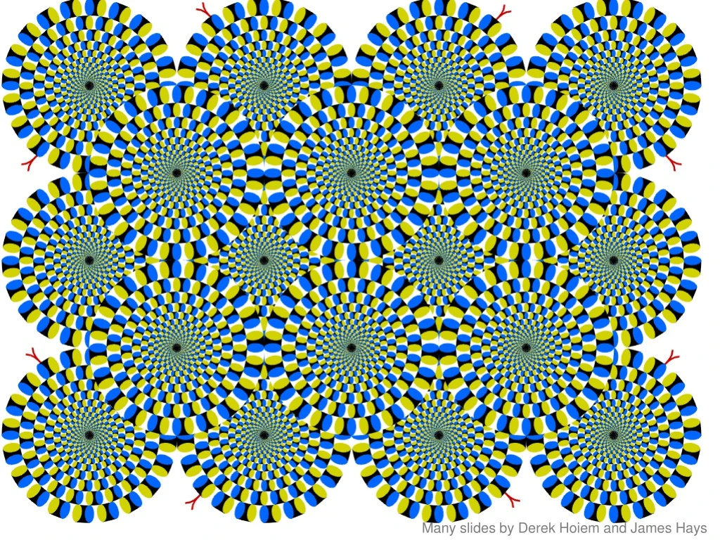
1. Motion illusion, rotating snakes Many slides by Derek Hoiem and James Hays

2. ProjectLive3D

3. Next two classes: views of filtering • Image filters in spatial domain • Filter is a mathematical operation of a grid of numbers • Smoothing, sharpening, measuring texture • Image filters in the frequency domain • Filtering is a way to modify the frequencies of images • Denoising, sampling, image compression • Templates and Image Pyramids • Filtering is a way to match a template to the image • Detection, coarse-to-fine registration

4. Image filtering • Image filtering: compute function of local neighborhood at each position • Really important! • Enhance images • Denoise, resize, increase contrast, etc. • Extract information from images • Texture, edges, distinctive points, etc. • Detect patterns • Template matching

5. Example: box filter 1 1 1 1 1 1 1 1 1 Slide credit: David Lowe (UBC)

6. Image filtering 1 1 1 1 1 1 1 1 1 Credit: S. Seitz

7. Image filtering 1 1 1 1 1 1 1 1 1 Credit: S. Seitz

8. Image filtering 1 1 1 1 1 1 1 1 1 Credit: S. Seitz

9. Image filtering 1 1 1 1 1 1 1 1 1 Credit: S. Seitz

10. Image filtering 1 1 1 1 1 1 1 1 1 Credit: S. Seitz

11. Image filtering 1 1 1 1 1 1 1 1 1 ? Credit: S. Seitz

12. Image filtering 1 1 1 1 1 1 1 1 1 ? Credit: S. Seitz

13. Image filtering 1 1 1 1 1 1 1 1 1 Credit: S. Seitz

14. Box Filter 1 1 1 1 1 1 1 1 1 • What does it do? • Replaces each pixel with an average of its neighborhood • Achieve smoothing effect (remove sharp features) Slide credit: David Lowe (UBC)

15. Smoothing with box filter

16. Practice with linear filters 0 0 0 0 1 0 0 0 0 ? Original Source: D. Lowe

17. Practice with linear filters 0 0 0 0 1 0 0 0 0 Original Filtered (no change) Source: D. Lowe

18. Practice with linear filters 0 0 0 0 0 1 0 0 0 ? Original Source: D. Lowe

19. Practice with linear filters 0 0 0 0 0 1 0 0 0 Original Shifted left By 1 pixel Source: D. Lowe

20. Practice with linear filters 0 1 0 1 0 1 1 0 2 1 0 1 1 0 1 0 0 1 - ? (Note that filter sums to 1) Original Source: D. Lowe

21. Practice with linear filters 0 1 0 1 0 1 1 0 2 1 0 1 1 0 1 0 0 1 - Original • Sharpening filter • Accentuates differences with local average Source: D. Lowe

22. Sharpening Source: D. Lowe

23. Other filters 1 0 -1 2 0 -2 1 0 -1 Sobel Vertical Edge (absolute value)

24. Other filters 1 2 1 0 0 0 -1 -2 -1 Sobel Horizontal Edge (absolute value)

25. Filtering vs. Convolution g=filter f=image • 2d filtering • h=filter2(g,f); or h=imfilter(f,g); • 2d convolution • h=conv2(g,f);

26. Key properties of linear filters Linearity: filter(f1 + f2) = filter(f1) + filter(f2) Shift invariance: same behavior regardless of pixel location filter(shift(f)) = shift(filter(f)) Any linear, shift-invariant operator can be represented as a convolution Source: S. Lazebnik

27. More properties • Commutative: a * b = b * a • Conceptually no difference between filter and signal • Associative: a * (b * c) = (a * b) * c • Often apply several filters one after another: (((a * b1) * b2) * b3) • This is equivalent to applying one filter: a * (b1 * b2 * b3) • Distributes over addition: a * (b + c) = (a * b) + (a * c) • Scalars factor out: ka * b = a * kb = k (a * b) • Identity: unit impulse e = [0, 0, 1, 0, 0],a * e = a Source: S. Lazebnik

28. Important filter: Gaussian • Weight contributions of neighboring pixels by nearness 0.003 0.013 0.022 0.013 0.003 0.013 0.059 0.097 0.059 0.013 0.022 0.097 0.159 0.097 0.022 0.013 0.059 0.097 0.059 0.013 0.003 0.013 0.022 0.013 0.003 5 x 5,  = 1 Slide credit: Christopher Rasmussen

29. Smoothing with Gaussian filter

30. Smoothing with box filter

31. Gaussian filters • Remove “high-frequency” components from the image (low-pass filter) • Images become more smooth • Convolution with self is another Gaussian • So can smooth with small-width kernel, repeat, and get same result as larger-width kernel would have • Convolving two times with Gaussian kernel of width σ is same as convolving once with kernel of width σ√2 • Separable kernel • Factors into product of two 1D Gaussians Source: K. Grauman

32. Separability of the Gaussian filter Source: D. Lowe

33. Separability example * = = * 2D convolution(center location only) The filter factorsinto a product of 1Dfilters: Perform convolutionalong rows: Followed by convolutionalong the remaining column: Source: K. Grauman

34. Separability • Why is separability useful in practice?

35. Some practical matters

36. Practical matters How big should the filter be? • Values at edges should be near zero • Rule of thumb for Gaussian: set filter half-width to about 3 σ

37. Practical matters • What about near the edge? • the filter window falls off the edge of the image • need to extrapolate • methods: • clip filter (black) • wrap around • copy edge • reflect across edge Source: S. Marschner

38. Practical matters Q? • methods (MATLAB): • clip filter (black): imfilter(f, g, 0) • wrap around: imfilter(f, g, ‘circular’) • copy edge: imfilter(f, g, ‘replicate’) • reflect across edge: imfilter(f, g, ‘symmetric’) Source: S. Marschner

39. Practical matters • What is the size of the output? • MATLAB: filter2(g, f, shape) • shape = ‘full’: output size is sum of sizes of f and g • shape = ‘same’: output size is same as f • shape = ‘valid’: output size is difference of sizes of f and g full same valid g g g g f f f g g g g g g g g Source: S. Lazebnik

40. Take-home messages 1 1 1 1 1 1 1 1 1 • Image is a matrix of numbers • Linear filtering is sum of dot product at each position • Can smooth, sharpen, translate (among many other uses) • Be aware of details for filter size, extrapolation, cropping =

41. Practice questions • Write down a 3x3 filter that returns a positive value if the average value of the 4-adjacent neighbors is less than the center and a negative value otherwise • Write down a filter that will compute the gradient in the x-direction: gradx(y,x) = im(y,x+1)-im(y,x) for each x, y

42. Practice questions Filtering Operator a) _ = D * B b) A = _ * _ c) F = D * _ d) _ = D * D 3. Fill in the blanks: A B E G C F D H I

43. Next: Thinking in Frequency

44. Why does the Gaussian give a nice smooth image, but the square filter give edgy artifacts? Gaussian Box filter

45. Hybrid Images • A. Oliva, A. Torralba, P.G. Schyns, “Hybrid Images,” SIGGRAPH 2006

46. Why do we get different, distance-dependent interpretations of hybrid images? ? Slide: Hoiem

47. Why does a lower resolution image still make sense to us? What do we lose? Image: http://www.flickr.com/photos/igorms/136916757/ Slide: Hoiem

48. Jean Baptiste Joseph Fourier (1768-1830) ...the manner in which the author arrives at these equations is not exempt of difficulties and...his analysis to integrate them still leaves something to be desired on the score of generality and even rigour. had crazy idea (1807): Any univariate function can be rewritten as a weighted sum of sines and cosines of different frequencies. • Don’t believe it? • Neither did Lagrange, Laplace, Poisson and other big wigs • Not translated into English until 1878! • But it’s (mostly) true! • called Fourier Series • there are some subtle restrictions Laplace Legendre Lagrange

49. A sum of sines Our building block: Add enough of them to get any signal f(x) you want!

50. Frequency Spectra • example : g(t) = sin(2πf t) + (1/3)sin(2π(3f) t) = + Slides: Efros