Download
1 / 44
440 likes | 607 Views
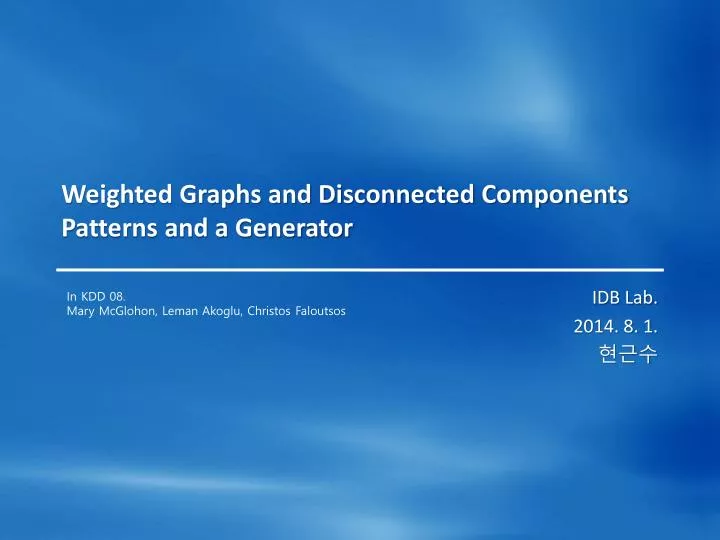
Weighted Graphs and Disconnected Components Patterns and a Generator. IDB Lab. 2014. 8 . 1. 현근수. In KDD 08. Mary McGlohon , Leman Akoglu , Christos Faloutsos. Outline. Introduction Related Work Data Observation Generative model Conclusion. “Disconnected” components.

E N D
Weighted Graphs and Disconnected ComponentsPatterns and a Generator IDB Lab. 2014. 8. 1. 현근수 In KDD 08. Mary McGlohon, Leman Akoglu, Christos Faloutsos
Outline • Introduction • Related Work • Data • Observation • Generative model • Conclusion
“Disconnected” components • In graphs a largest connected component emerges. • What about the smaller-size components? • How do they emerge, and join with the large one?
Weighted edges • Graphs have heavy-tailed degree distribution. • What can we also say about these edges? • How are they repeated, or otherwise weighted?
Goals • Observe “Next-largest connected components(NLCCs)” Q1. How does the GCC emerge? Q2. How do NLCC’s emerge and join with the GCC? • Find properties that govern edge weights Q3: How does the total weight of the graph relate to the number of edges? Q4: How do the weights of nodes relate to degree? Q5: Does this relation change with the graph? • Q6: Can we produce an emergent, generative model
Properties of networks • Small diameter (“small world” phenomenon) • [Milgram 67] [Leskovec, Horovitz 07] • Heavy-tailed degree distribution • [Barabasi, Albert 99] [Faloutsos, Faloutsos, Faloutsos 99] • Densification • [Leskovec, Kleinberg, Faloutsos 05] • “Middle region” components as well as GCC and singletons • [Kumar, Novak, Tomkins 06]
Generative Models • Erdos-Renyi model [Erdos, Renyi 60] • Preferential Attachment [Barabasi, Albert 99] • Forest Fire model [Leskovec, Kleinberg, Faloutsos 05] • Kronecker multiplication [Leskovec, Chakrabarti, Kleinberg, Faloutsos 07] • Edge Copying model [Kumar, Raghavan, Rajagopalan, Sivakumar, Tomkins, Upfal 00] • “Winners don’t take all” [Pennock, Flake, Lawrence, Glover, Giles 02]
Diameter • Diameter of a graph is the “longest shortest path” • Effective diameter is the distance at which 90% of nodes can be reached. diameter=3 n5 n1 n2 n6 n3 n4 n7
Unipartite Networks • Postnet: Posts in blogs, hyperlinks between • Blognet: Aggregated Postnet, repeated edges • Patent: Patent citations • NIPS: Academic citations • Arxiv: Academic citations • NetTraffic: Packets, repeated edges • Autonomous Systems (AS): Packets, repeated edges (3) n1 n3 n2 n4 n5 n6 n7
Unipartite Networks • Postnet: Posts in blogs, hyperlinks between • Blognet: Aggregated Postnet, repeated edges • Patent: Patent citations • NIPS: Academic citations • Arxiv: Academic citations • NetTraffic: Packets, repeated edges • Autonomous Systems (AS): Packets, repeated edges 10 1.2 n1 n3 1 n2 8.3 6 n4 2 n5 n6 n7
Unipartite Networks • (Nodes, Edges, Timestamps) • Postnet: 250K, 218K, 80 days • Blognet: 60K,125K, 80 days • Patent: 4M, 8M, 17 yrs • NIPS: 2K, 3K, 13 yrs • Arxiv: 30K, 60K, 13 yrs • NetTraffic: 21K, 3M, 52 mo • AS: 12K, 38K, 6 mo n1 n3 n2 n4 n5 n6 n7
Bipartite Networks • IMDB: Actor-movie network • Netflix: User-movie ratings • DBLP: repeated edges • Author-Keyword • Keyword-Conference • Author-Conference • US Election Donations: $ weights, repeated edges • Orgs-Candidates • Individuals-Orgs n1 m1 n2 m2 n3 m3 n4
Bipartite Networks • IMDB: Actor-movie network • Netflix: User-movie ratings • DBLP: repeated edges • Author-Keyword • Keyword-Conference • Author-Conference • US Election Donations: $ weights, repeated edges • Orgs-Candidates • Individuals-Orgs 10 n1 1.2 m1 2 n2 5 m2 1 n3 6 m3 n4
Bipartite Networks • IMDB: 757K, 2M, 114 yr • Netflix: 125K, 14M, 72 mo • DBLP: 25 yr • Author-Keyword: 27K, 189K • Keyword-Conference: 10K, 23K • Author-Conference: 17K, 22K • US Election Donations: 22 yr • Orgs-Candidates: 23K, 877K • Individuals-Orgs: 6M, 10M n1 m1 n2 m2 n3 m3 n4
Observation 1: Gelling Point Q1: How does the GCC emerge?
Observation 1: Gelling Point • Most real graphs display a gelling point, or burning off period • After gelling point, they exhibit typical behavior. This is marked by a spike in diameter. IMDB t=1914 Diameter Time
Observation 2: NLCC behavior Q2: How do NLCC’s emerge and join with the GCC? Do they continue to grow in size? Do they shrink? Stabilize?
Observation 2: NLCC behavior • After the gelling point, the GCC takes off, but NLCC’s remain constant or oscillate. IMDB CC size Time
Observation 3 Q3: How does the total weight of the graph relate to the number of edges?
Observation 3: Fortification Effect • $ = # checks ? Orgs-Candidates 2004 |$| 1980 |Checks|
Observation 3: Fortification Effect • Weight additions follow a power law with respect to the number of edges: • W(t): total weight of graph at t • E(t): total edges of graph at t • w is PL exponent • 1.01 < w < 1.5 = super-linear! • (more checks, even more $) Orgs-Candidates 2004 |$| 1980 |Checks|
Observation 4 and 5 Q4: How do the weights of nodes relate to degree? Q5: Does this relation change over time?
Observation 4: Snapshot Power Law • At any time, total incoming weight of a node is proportional to in degree with PL exponent, iw. 1.01 < iw < 1.26, super-linear • More donors, even more $ Orgs-Candidates e.g. John Kerry, $10M received, from 1K donors In-weights ($) Edges (# donors)
Observation 5:Snapshot Power Law • For a given graph, this exponent is constant over time. Orgs-Candidates exponent Time
Goals of model • a) Emergent, intuitive behavior • b) Shrinking diameter • c) Constant NLCC’s • d) Densification power law • e) Power-law degree distribution
Goals of model • a) Emergent, intuitive behavior • b) Shrinking diameter • c) Constant NLCC’s • d) Densification power law • e) Power-law degree distribution = “Butterfly” Model
Butterfly model in action • A node joins a network, with own parameter. pstep n8 “Curiosity” n1 n3 n2 n4 n5 n6 n7
Butterfly model in action • A node joins a network, with own parameter. • With (global) phost, chooses a random host phost “Cross-disciplinarity” n8 n1 n3 n2 n4 n5 n6 n7
Butterfly model in action • A node joins a network, with own parameters. • With (global) phost, chooses a random host • With (global) plink, creates link plink “Friendliness” n8 n1 n3 n2 n4 n5 n6 n7
Butterfly model in action • A node joins a network, with own parameters. • With (global) phost, chooses a random host • With (global) plink, creates link • With pstep travels to random neighbor n8 n1 pstep n3 n2 n4 n5 n6 n7
Butterfly model in action • A node joins a network, with own parameters. • With (global) phost, chooses a random host • With (global) plink, creates link • With pstep travels to random neighbor. Repeat. n8 n1 n3 plink n2 n4 n5 n6 n7
Butterfly model in action • A node joins a network, with own parameters. • With (global) phost, chooses a random host • With (global) plink, creates link • With pstep travels to random neighbor. Repeat. n8 n1 n3 pstep n2 n4 n5 n6 n7
Butterfly model in action • Once there are no more “steps”, repeat “host” procedure: • With phost, choose new host, possibly link, etc. n8 phost n1 n3 n2 n4 n5 n6 n7
Butterfly model in action • Once there are no more “steps”, repeat “host” procedure: • With phost, choose new host, possibly link, etc. n8 phost n1 n3 n2 n4 n5 n6 n7
Butterfly model in action • Once there are no more “steps”, repeat “host” procedure: • With phost, choose new host, possibly link, etc. • Until no more steps, and no more hosts. n8 n1 plink n3 n2 n4 n5 n6 n7
Butterfly model in action • Once there are no more “steps”, repeat “host” procedure: • With phost, choose new host, possibly link, etc. • Until no more steps, and no more hosts. n8 n1 n3 pstep n2 n4 n5 n6 n7
a) Emergent, intuitive behavior Novelties of model: • Nodes link with probability • May choose host, but not link (start new component) • Incoming nodes are “social butterflies” • May have several hosts (merges components) • Some nodes are friendlier than others • pstep different for each node • This creates power-law degree distribution (theorem)
Validation of Butterfly • Chose following parameters: • phost= 0.3 • plink = 0.5 • pstep ~ U(0,1) • Ran 10 simulations • 100,000 nodes per simulation
b) Shrinking diameter • Shrinking diameter • In model, gelling usually occurred around N=20,000 N=20,000 Diam- eter Nodes
c) Oscillating NLCC’s • Constant / oscillating NLCC’s N=20,000 NLCC size Nodes
d) Densification power law • Densification: • Our datasets had a=(1.03, 1.7) • In [Leskovec+05-KDD], a= (1.1, 1.7) • Simulation produced a = (1.1,1.2) Edges N=20,000 Nodes
e) Power-law degree distribution • Power-law degree distribution • Exponents approx -2 Count Degree
Summary • Studied several diverse public graphs • Measured at many timestamps • Unipartite and bipartite • Blogs, citations, real-world, network traffic • Largest was 6 million nodes, 10 million edges
Summary • Observations on unweighted graphs: A1: The GCC emerges at the “gelling point” A2: NLCC’s are of constant / oscillating size • Observations on weighted graphs: A3: Total weight increases super-linearly with edges A4: Node’s weights increase super-linearly with degree, power law exponent iw A5: iw remains constant over time • A6: Intuitive, emergent generative “butterfly” model, that matches properties