FORMAL METHODS IN HARDWARE VERIFICATION

1. FORMAL METHODS IN HARDWARE VERIFICATION Maciej Ciesielski Dept. of Electrical & Computer Engineering University of Massachusetts, Amherst, USA ciesiel@ecs.umass.edu Formal Verification

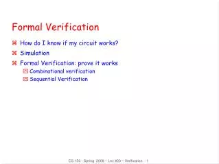
2. Overview • Introduction • What is verification (validation) • Why do we need it • Formal verification vs. simulation-based methods • Math background • Decision diagrams (BDD’s, BMD’s, etc.) • Symbolic FSM traversal • Formal methods • model checking • equivalence checking • Semi-formal methods • symbolic simulation • functional validation Formal Verification

3. Formal Methods • Equivalence checking • Combinational circuits • Sequential circuits • Model checking • Problem statement • Explicit algorithms (on graphs) • Symbolic algorithms (using BDDs) • Theorem proving • Deductive reasoning Formal Verification

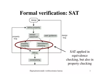
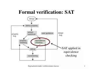
4. Functional Testing • Simulation-based methods • Symbolic simulation • Functional test generation • SAT-based methods, Boolean SAT • RTL verification: Arithmetic/Boolean SAT • ATPG-based methods • Emulation-based methods • Hardware-assisted simulation • System prototyping Formal Verification

5. Part I INTRODUCTION Formal Verification

6.  ? model Design 1 Design 2  ? RTL HDL / RTL behavior  ? Logic level Logic level function  ?  ?  ? structure Gate level Gate level  ? layout Mask level Mask level Verification • Design verification = ensuring correctness of the design • against its implementation (at different levels) • against alternative design (at the same level) Formal Verification

7. Why Verification • Verification crisis • System complexity, difficult to manage • More time, effort devoted to verification than to actual design • Need automated verification methods, integration • Consequences • Disasters, life threatening situations • Inconvenience (Pentium bug … ?) • Many more … Formal Verification

8. Formal Verification Verification Methods • Deductive verification • Model checking • Equivalence checking • Simulation - performed on the model • Emulation, prototyping – product + environment • Testing - performed on the actual product (manufacturing test) Formal Verification

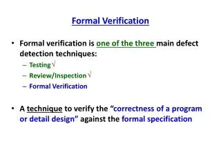
9. Formal Verification • Deductive reasoning (theorem proving) • uses axioms, rules to prove system correctness • no guarantee that it will terminate • difficult, time consuming: for critical applications only • Model checking • automatic technique to prove correctness of concurrent systems: digital circuits, communication protocols, etc. • Equivalence checking • check if two circuits are equivalent • OK for combinational circuits, unsolved for sequential Formal Verification

10. Why Formal Verification • Need for reliable hardware validation • Simulation, test cannot handle all possible cases • Formal verification conducts exhaustive exploration of all possible behaviors • compare to simulation, which explores some of possible behaviors • if correct, all behaviors are verified • if incorrect, a counter-example (proof) is presented • Examples of successful use of formal verification • SMV system [McMillan 1993] • verification of cache coherence protocol in IEEE Futurebus+ standard Formal Verification

11. Model Checking • Algorithmic method of verifying correctness of (finite state) concurrent systems against temporal logic specifications • A practical approach to formal verification • Basic idea • System is described in a formal model • derived from high level design (HDL, C), circuit structure, etc. • The desired behavior is expressed as a set of properties • expressed as temporal logic specification • The specification is checked against the model Formal Verification

12. Functional Validation • Verify the design in the full operational context • RTL functional verification • Validate HDL specification of RTL model • Functional test generation • SAT-based methods (Boolean, arithmetic) • ATPG-based methods • Symbolic simulation (semi-formal methods) • Combine simulation with symbolic methods Formal Verification

13. Part IIBACKGROUND • Canonical representations: BDD, BMD • Boolean satisfiability problem (SAT) • Finite State Machine (FSM) traversal Formal Verification

14. Binary Decision Diagrams (BDD) • Based on recursive Shannon expansion F = x Fx + x’ Fx’ • Compact data structure for Boolean logic • can represents sets of objects (states) encoded as Boolean functions • Canonical representation • reduced ordered BDDs (ROBDD) are canonical • essential for verification Formal Verification

15. b b a a b b f f f c 0 0 1 1 BDD Construction • Typically done using APPLY operator • Reduction rules • remove duplicate terminals • merge duplicate nodes (isomorphic subgraphs) • remove redundant nodes • Redundant nodes: • nodes with identical children Formal Verification

16. f 1 edge a b c f 0 0 0 0 0 0 1 0 0 1 0 0 0 1 1 1 1 0 0 0 1 0 1 1 1 1 0 0 1 1 1 1 0 edge a b b c c c c 0 0 0 0 0 1 1 1 BDD Construction – your first BDD • Construction of a Reduced Ordered BDD f = ac + bc Truth table Decision tree Formal Verification

17. f f a a a b b b b b c c c c c c c 0 0 0 1 1 1 BDD Construction – cont’d f = (a+b)c 1. Remove duplicate terminals • 2. Merge duplicate nodes 3. Remove redundant nodes Formal Verification

18. a a b b c c 0 0 1 1 Application to Verification • Equivalence of combinational circuits • Canonicity property of BDDs: • if F and G are equivalent, their BDDs are identical (for the same ordering of variables) F = a’bc + abc +ab’c G = ac +bc  Formal Verification

19. a ab b c 1 0 ab’c Application to Verification, cont’d • Functional test generation • SAT, Boolean satisfiability analysis • to test for H = 1 (0), find a path in the BDD to terminal 1 (0) • the path, expressed infunction variables, gives a satisfying solution (test vector) H Formal Verification

20. F F’ ¬ F(y) F(x,y) Restrict x=b 0 0 1 0 0 1 1 1 Logic Manipulation using BDDs • Useful operators • Complement ¬ F = F’ • (switch the terminal nodes) • Restrict: F|x=b = F(x=b) where b = const Formal Verification

21.   F G G F =   0 0 1 1 0 1 Useful BDD Operators - cont’d • Apply: F G where stands for any Boolean operator (AND, OR, XOR, ) • Any logic operation can be expressed using only Restrict and Apply • Efficient algorithms, work directly on BDDs Formal Verification

22. Apply Operation • Basic operator for efficient BDD manipulation (structural) • Based on recursive Shannon expansion F OP G = x (FxOP Gx) + x’(Fx’OP Gx’) whereOP = OR, AND, XOR, etc Formal Verification

23. 2 a a 3 2.3 1.3 c c 1.0 0.3 0 0 0 1.1 1 1 1 Apply Operation - AND a AND c ac a = = c AND Formal Verification

24. ac bc 4 a 6 b a a b 5 7 b 7+5 0+6 6+5 4+6 0+7 0+5 c c c c 0+0 0 0 0 0 1 1 1 1 Apply Operation - OR f = ac+bc OR = = Formal Verification

25. Binary Moment Diagrams (*BMD) • Devised for word-level operations, arithmetic • Based on Shannon expansion, manipulated f = x fx + x’ fx’ = x fx + (1-x) fx’ = fx’ + x (fx - fx’ ) = fx’ + x fx. • fx’ = f(x=0),is constant (zero moment) • fx. = (fx - fx’ ) is called first moment, similar to first derivative • Additive and multiplicative weights on edges (*BMD) Formal Verification

26. 4 2 4 1 2 1 4 4 0 0 0 0 1 1 1 1 x2 x1 x1 x0 x0 x2 y2 y1 y0 y2 y1 y0 Y X Y X 2 2 1 1 word level word level Bit level Bit level *BMD for arithmetic circuits • Efficiently models word-level operators X Y X + Y Formal Verification

27. x x x x x y = x y x  y = (x + y – x y) x  y = (x + y – 2 x y) x’ = (1-x) 1 -1 y y y y y 0 0 0 0 1 1 1 1 -1 -2 1 1 NOT XOR AND OR *BMD for Boolean logic • Needed to model complex arithmetic circuits Formal Verification

28. Decison Diagrams - summary • BDDs and BMDs are canonical for fixed variable order • BDDs • Good for equivalence checking and SAT • Inefficient for large arithmetic circuits (multipliers) • BMDs • Efficient for word-level operators • Less compact for Boolean logic than BDDs • Good for equivalence checking, but not for SAT • New type of compact, canonical diagram available, better suited for arithmetic designs • TED, based on Taylor series Expansion Formal Verification

29. Boolean Satisfiability (SAT) • Given a representation for a Boolean function f (X): • Find an assignment X* such that f (X*) = 1, or • Prove that such an assignment does not exist • A classical way to solve SAT: • Represent function f (X) in conjunctive normal form (CNF) • Solve SAT by finding satisfying assignment to binary variables for each clause (GRASP, SATO) Formal Verification

30. a d b CNF for Boolean Network • Represent Boolean function as a connection of gates • Represent each gate as a CNF clause • Solve = find satisfying assignment for all CNF clauses jd= [d = ¬(a b )][¬d = a b] = [d =¬a +¬b][¬d = a b] = (¬a ® d)(¬b ® d)(a b ®¬d) = (a +d)(b +d)(¬a +¬b + ¬d) Formal Verification

31. O X (s,x) (s,x) s s’ R Finite State Machines (FSM) • FSM M(X,S, , ,O) • Inputs: X • Outputs: O • States: S • Next state function, (s,x) : S  X  S • Output function, (s,x) : S X  O Formal Verification

32. 1/0 0/1 s0 s1 s2 1/0 0/1 FSM Traversal • State Transition Graphs • directed graphs with labeled nodes and arcs (transitions) • symbolic state traversal methods • important for symbolic verification, state reachability analysis, FSM traversal, etc. 0/0 Formal Verification

33. Existential Quantification • Existential quantification (abstraction) xf = f |x=0+ f |x=1 • Example: x(x y + z) = y + z • Note: xf does not depend on x (smoothing) • Useful in symbolic image computation (sets of states) Formal Verification

34. Existential Quantification - cont’d • Function can be existentially quantified w.r.to a vector: X = x1x2… Xf = x1x2...f = x1 x2 ...f • Can be done efficiently directly on a BDD • Very useful in computing sets of states • Image computation: next states • Pre-Image computation: previous states from a given set of initial states Formal Verification

35. R(u,v) S(u) Img(v) Image Computation • Computing set of next states from a given initial state (or set of states) Img( S,R ) = uS(u)• R(u,v) • FSM: when transitions are labeled with input predicates x, quantify w.r.to all inputs (primary inputs and state var) • Img( S,R ) = x uS(u)• R(x,u,v) Formal Verification

36. s2 a a xy XY 01 s1 s4 1 0001 0 0010 - 1011 ………. 00 a’ 11 10 s3 Image Computation - example Compute a set of next states from state s1 • Encode the states: s1=00, s2=01, s3=10, s4=11 • Write transition relations for the encoded states: R = (ax’y’X’Y + a’x’y’XY’ + xy’XY + ….) Formal Verification

37. s2 a 01 s1 s4 00 a’ 11 10 s3 Example - cont’d • Compute Image from s1 under R Img( s1,R ) = a xy s1(x,y) • R(a,x,y,X,Y) =a xy(x’y’)• (ax’y’X’Y + a’x’y’XY’ + xy’XY + ….) = axy(ax’y’X’Y + a’x’y’XY’ ) = (X’Y + XY’) = {01, 10} = {s2,s3} Result: a set of next states for all inputs s1  {s2, s3} Formal Verification

38. R(u,v) S’(v) Pre-Img(u) Pre-Image Computation • Computing a set of present states from a given next state (or set of states) Pre-Img( S’,R) = vR(u,v) )• S’(v) • Similar to Image computation, except that quantification is done w.r.to next state variables • The result: a set of states backward reachable from state set S’, expressed in present state variables u • Useful in computing CTL formulas: AF, EF Formal Verification

39. Part IIIEQUIVALENCE CHECKING Formal Verification

40. Out In CL PI Po CL Ps Ns R Equivalence Checking • Two circuits are functionally equivalent if they exhibit the same behavior • Combinational circuits • for all possible input values • Sequential circuits • for all possible input sequences Formal Verification

41. Combinational Equivalence Checking • Functional Approach • transform output functions of combinational circuits into a unique (canonical) representation • two circuits are equivalent if their representations are identical • efficient canonical representation: BDD • Structural • identify structurally similar internal points • prove internal points (cut-points) equivalent • find implications Formal Verification

42. Functional Equivalence • If BDD can be constructed for each circuit • represent each circuit as shared (multi-output) BDD • use the same variable ordering ! • BDDs of both circuits must be identical • If BDDs are too large • cannot construct BDD, memory problem • use partitioned BDD method • decompose circuit into smaller pieces, each as BDD • check equivalence of internal points Formal Verification

43. F G f2 g2 z z f1 g1 y y x x Functional Decomposition • Decompose each function into functional blocks • represent each block as a BDD (partitionedBDD method) • define cut-points (z) • verify equivalence of blocks at cut-points starting at primary inputs Formal Verification

44. F G f2 g2 z1 z2 f1 g1 y y x x Cut-Points Resolution Problem • If all pairs of cut-points (z1,z2) are equivalent • so are the two functions, F,G • If intermediate functions (f2,g2) are not equivalent • the functions (F,G) may still be equivalent • this is called false negative • Why do we have false negative ? • functions are represented in terms of intermediate variables • to prove/disprove equivalence must represent the functions in terms of primary inputs (BDD composition) Formal Verification

45. F G f2 g2 z z f1 g1 y y x x Cut-Point Resolution – Theory • Let f1(x)=g1(x) x • if f2(z,y)  g2(z,y), z,y then f2(f1(x),y)  g2(f1(x),y)  F  G • if f2(z,y)  g2(z,y), z,y  f2(f1(x),y)  g2(f1(x),y)  F  G We cannot say ifF  G or not • False negative • two functions are equivalent, but the verification algorithm declares them as different. Formal Verification

46. 0, F  G (false negative) 1, F  G (true negative) F G Cut-Point Resolution – cont’d • How to verify if negative is false or true ? • Procedure 1: create a miter (XOR) between two potentially equivalent nodes/functions • perform ATPG test for stuck-at 0 • find test pattern to prove F  G • efiicient for true negative (gives test vector, a proof) • inefficient when there is no test Formal Verification

47. , F  G (false negative) Non-empty, F  G G F F G =  = Cut-Point Resolution – cont’d • Procedure 2: create a BDD for F G • perform satisfiability analysis (SAT) of the BDD • if BDD for FG = , problem is not satisfiable, false negative • BDD for FG, problem is satisfiable, true negative Note: must compose BDDs until they are equivalent, or expressed in terms of primary inputs • the SAT solution, if exists, provides a test vector (proof of non-equivalence) – as in ATPG • unlike the ATPG technique, it is effective for false negative (the BDD is empty!) Formal Verification

48. d1 d2 a F G • a • b b c Structural Equivalence Check • Given two circuits, each with its own structure • identify “similar” internal points, cut sets • exploit internal equivalences • False negative problem may arise • F  G, but differ structurally (different local support) • verification algorithm declares F,G as different • Solution: use BDD-based or ATPG-based methods to resolve the problem. Also: implication, learning techniques. Formal Verification

49. d=x b=x f=1 a=0 d=0 b=x f=0 c=x e=x a=1 c=x e=0 Implication Techniques • Techniques that extract and exploit internal correspondences to speed up verification • Implications – direct and indirect Direct: a=1  f=0 Indirect (learning): f=1  a=0 Formal Verification

50. G H a a a H=? b b b G=1 c 0 1 0 1 Learning Techniques • Learning • process of deriving indirect implications • Recursive learning • recursively analyzes effects of each justification • Functional learning • uses BDDs to learn indirect implications G=1  H=0 Formal Verification