Download
1 / 30
300 likes | 504 Views
Production. APEC 3001 Summer 2007 Readings: Chapter 9 &Appendix in Frank. Objectives. Describing Production Short-Run Production Long-Run Production Returns to Scale. Describing Production Definitions. Output: Good or service produced by an individual or firm. Inputs:

E N D
Production APEC 3001 Summer 2007 Readings: Chapter 9 &Appendix in Frank
Objectives • Describing Production • Short-Run Production • Long-Run Production • Returns to Scale
Describing ProductionDefinitions • Output: • Good or service produced by an individual or firm. • Inputs: • Resources used in the production of output. • Production Function: • A relationship that describes how inputs can be transformed into output. • e.g. Q = F(K,L) where K is capital & L is labor. • Intermediate Product: • Products that are transformed by a production process into products of greater value.
InputsDefinitions • Variable Inputs: • Inputs in a production process that can be changed. • Fixed Inputs: • Inputs in a production process that can not be changed.
Short-Run ProductionDefinitions & Example • Definition • The longest period of time during which at least one of the inputs used in the production process cannot be varied. • Example • Suppose K = K0, such that Q = F(K0,L) = F0(L). • Output in the short-run only depends on the amount of labor we choose. • Some More Definitions • Total Product Curve: • A curve showing the amount of output as a function of the amount of variable input. • Law of Diminishing Returns: • If other inputs are fixed, the increase in output from an increase in variable inputs must eventually decline.
Typical Short Run Production Function or Total Product Curve Output (Q) Q = F(K0, L) 0 L0 L1 Variable Input (L)
Short-Run ProductionRegions of Production • Region I: • Increasing Returns - 0 to L0 • Region II: • Decreasing (Positive) Returns - L0 to L1 • Region III: • Decreasing (Negative) Returns - Above L1 The Law of Diminishing Returns means that Region II must exist.
Short-Run ProductionMore Definitions • Marginal Product: • Change in total product due to a one-unit change in the variable input: MPL = Q/L = F0’(L). • Average Product: • Total output divided by the quantity of the variable input: APL = Q/L = F0(L)/L. • Example • Suppose Q = KL2 and K0 = 100. • F0(L) = 100L2 • MPL = 200L • APL = 100L2/L = 100L
Marginal Product Curve Output (Q) 0 L0 L1 MPL Variable Input (L)
Short-Run ProductionProduction Regions & Marginal Products • Region I: • Increasing Marginal Product - 0 to L0 • Region II: • Decreasing (Positive) Marginal Product - L0 to L1 • Region III: • Decreasing (Negative) Marginal Product - Above L1
Calculation of Average Product Output (Q) APL = Q/L = (Q0 – 0) / (L0 – 0) = Q0 / L0 Q0 Q = F(K0, L) L0 0 Variable Input (L)
Total Product Curve and Maximum Average Product Output (Q) Maximum APL = Q2 / L2 Q2 Q = F(K0, L) 0 L0 L2 L1 Variable Input (L)
Marginal and Average Product Curves Output (Q) APL 0 L0 L2 L1 MPL Variable Input (L)
Relationship Between Marginal & Average Products • MPL > APL APL is increasing (e.g. below L2). • MPL < APL APL is decreasing (e.g. above L2). • MPL = APL APL is maximized (e.g. at L2).
Long-Run Production • Definition • The shortest period of time required to alter the amount of all inputs used in a production process. • Assumptions • Regularity • Monotonicity • Convexity
Regularity • There is some way to produce any particular level of output. Similar to the completenessassumption for rational choice theory.
Monotonicity • If it is possible to produce a particular level of output with a particular combination of inputs, it is also possible to produce that level of output when we have more of some inputs. Similar to the more-is-better assumption for rational choice theory.
Convexity • If it is possible to produce a particular level of output with either of two different combinations of inputs, then it is also possible to produce that level of output with a mixture of the two combinations of inputs. Similar to the convexity assumption for rational choice theory. These assumptions imply that we have very specific production possibilities!
Figure 6: Production Possibilities Input Combinations Capable of Producing Q0 This is not enough! Q0
Region A: Input Combinations Capable of Producing Q0 Region B: Input Combinations Capable of Producing Q0 & Q1 Region B Region A Q1 Q0
The Problem • Combinations of capital & labor in region A are capable of producing Q0. • Combinations of capital & labor in region B are capable of producing Q1 & Q0. • Without being more specific, the production function will not yield a unique output for different combinations of capital & labor. • Question: What other assumptions can we make to be sure a combination of capital & labor gives us a unique level of output? • We can assume production is efficient!
We can use combination B to produce Q0, but we would not be doing the best we can with what we have! We can use combination A to produce Q0, and we would be doing the best we can with what we have! B A Q0
Regularity, Monotonicity, Convexity, & Efficiency • We can construct a production function: Q = F(K,L). • Unlike the utility function, the production function is cardinal. • 2,000 Units of Output is Twice as Much as 1,000 • Definitions • Isoquant: • The set of all efficient input combinations that yield the same level of output. • Isoquant map: • A representative sample of the set of a firm’s isoquants used as a graphical summary of production.
Properties of Isoquants & Isoquant Maps • Higher Isoquants (Isoquants to the Northeast) represent higher levels of output. • Ubiquitous • Downward Sloping • Cannot Cross • Become Less Steep Moving Down & Right (Bowed Toward the Origin)
Figure 7: Example Isoquant Map Q=30 Q=20 Q=10
Marginal Rate of Technical Substitution (MRTS) • Definition: • The rate at which one input can be exchanged for another without altering the total level of output: |K/L| = MPL/MPK =
Figure 8: Marginal Rate of Technical Substitution MRTS of Capital for Labor at A= |K/L| A K L Q=20
Returns to ScaleDefinitions • Increasing Returns to Scale: • A proportional increase in every input yields more than a proportional increase in output. • Constant Returns to Scale: • A proportional increase in every input yields an equal proportional increase in output. • Decreasing Returns to Scale: • A proportional increase in every input yields less than a proportional increase in output.
Identifying Returns to Scale • Let > 1 • If Q < F(K, L), returns to scale are increasing. • If Q = F(K, L), returns to scale are constant. • If Q > F(K, L), returns to scale are decreasing. • Example • Suppose Q = F(K,L) = KaLb. • Then F(K, L) = (K)a(L)b = aKabLb = a+bKaLb = a+bQ • a + b > 1 Q < a+bQ or increasing returns to scale. • a + b = 1 Q = a+bQ or constant returns to scale. • a + b < 1 Q > a+bQ or decreasing returns to scale.
What You Should Know • What a production function is? • Short-Run versus Long Run Production • Short-Run Production • Total Product, Marginal Product, & Average Product • Law of Diminishing Returns • Long-Run Production • Assumptions • Isoquants & Isoquant Maps: What they are & properties. • Marginal Rate of Technical Substitution • Returns to Scale: What they are and how to test.