Download
1 / 15
150 likes | 278 Views
Distributed Computation of a Sparse Matrix Vector Product. Lecture 18 MA/CS 471 Fall 2003. So Far. We have so far discussed: We discovered (by constructing the iteration for the error vector) that the convergence rate was determined by the spectral radius of:

E N D
Distributed Computation of a Sparse Matrix Vector Product Lecture 18 MA/CS 471 Fall 2003
So Far • We have so far discussed: • We discovered (by constructing the iteration for the error vector) that the convergence rate was determined by the spectral radius of: • The smaller the spectral radius of this matrix the faster the convergence rate..
Parallel Implementation • A further consideration over which scheme to use is the relative parallel efficiency. • We noted by demonstration that Gauss-Seidel appears to be much less “parallel” than Jacobi iteration..
Non-Stationnary Methods • There are many alternative approaches to solving • We will consider a set of Krylov sub-space methods. • Specifically the popular conjugate gradient method for symmetric, positive definite A.
Basic Idea • One can view the solution of Ax=b as a minimization problem. • We define the quadratic form: • We will show that if A is positive-definite and symmetric then the solution of Ax=b minmizes f See: http://www-2.cs.cmu.edu/~jrs/jrspapers.html#cg
Minimizer of f • In order to find minima of the quadratic form function f we can take a gradient with respect to x • If A is symmetric then: Do demonstration on board.
cont • So if A is symmetric then at a minimum of f • i.e. the system we wish to solve. • Thus the solution to Ax=b is a critical point of f • Next we show that if A is positive-definite then this critical point is a global minimum..
Global Minimum • We consider the difference between f at the solution x and any other vector p:
Summary So Far • If A is symmetric, positive definite then • Has a global minimum at the solution to Ax=b • Approach: use a minimization algorithm to iterate towards the global minimizer.
Conjugate-Gradient • This algorithm is suitable for solving Ax=b where A is symmetric and positive-definite.
Conjugate-Gradient Algorithm • Sequence: See: http://www-2.cs.cmu.edu/~jrs/jrspapers.html#cg
Parallel Implementation • There are a few bottlenecks • Any dot product will requirea global all reduce. • The norm of the residual requires a global all-reduce.
Rate of Convergence • Definition: • The error equation (after a lot of work) now looks like: • i.e. in the problem induced A norm, the error will decay by a factor at each iteration which is determined by a function of the spectral condition number (kappa)
cont • So we can note that the larger the spectral condition of the matrix A the more iterations it can take