Download
1 / 22
220 likes | 227 Views
Modern Control Systems (MCS). Lecture-41-42 Design of Control Systems in Sate Space Quadratic Optimal Control. Dr. Imtiaz Hussain email: imtiaz.hussain@faculty.muet.edu.pk URL : http://imtiazhussainkalwar.weebly.com/. Outline. Introduction Quadratic Cost Function

E N D
Modern Control Systems (MCS) Lecture-41-42 Design of Control Systems in Sate Space Quadratic Optimal Control Dr. Imtiaz Hussain email: imtiaz.hussain@faculty.muet.edu.pk URL :http://imtiazhussainkalwar.weebly.com/
Outline • Introduction • Quadratic Cost Function • Optimal Control System based on Quadratic Performance Index • Optimization by Second Method of Liapunov • Quadratic Optimal Control • Examples
Introduction • Optimization is the selection of a best element(s) from some set of available alternatives. • In control Engineering, optimization means minimizing a cost function by systematically choosing parameter values from within an allowed set of tunable parameters. • Acost function orloss function or performance indexis a function that maps an event or values of one or more variables onto a real number intuitively representing some "cost" associated with the event (e.g. error function).
Quadratic Cost Function • The use of a quadratic loss function is common, for example when using least squares techniques. • It is often more mathematically tractable than other loss functions because of the properties of variances, as well as being symmetric: an error above the target causes the same loss as the same magnitude of error below the target. • If the target is , then quadratic loss function is given as • Where is the actual value.
Optimal Control System based on Quadratic Performance Index • In many practical control systems, we desire to minimize some function of error signal. • For example, given a system • We may wish to minimize a generalized error function such as • Where represents the desired state, actual state, and Q a positive definite real symmetric matrix.
Optimal Control System based on Quadratic Performance Index • In addition to considering error as a measure of system performance we also must pay attention to the energy required for control action. • Since the control signal may have the dimension of force or torque, the control energy is proportional to the integral of such control signal squared. • Where R is a positive definite real symmetric matrix. • The performance index of a control system over the time interval may then be written, with the use of Lagrange multiplier , as
Optimal Control System based on Quadratic Performance Index • If and desired state is the origin () then • It is called the quadratic performance index. • Note that the choice of weighting matrices Q and R is in a sense arbitrary. • A regulator system designed by minimizing a quadratic performance index is called a quadratic optimal regulator system. • This approach is alternative to the pole-placement approach for the design of stable regulator systems.
Optimization by Second Method of Liapunov • We will drive a direct relationship between Liapunov function and quadratic performance index and solve the optimization problem using this relationship. • Let us consider the system • Where is an asymptotically stable equilibrium state. We assume that matrix A involve an adjustable parameter (or parameters). • It is desired to minimize the following performance index. • The problem thus becomes that of determining the value(s) of adjustable parameter(s) so as to minimize the performance index.
Optimization by Second Method of Liapunov • We know from Liapunov stability theorem (Lecture-39-40) that • The performance index J can be evaluated as
Optimization by Second Method of Liapunov • Since the system has stable equilibrium state at the origin of state space therefore • Thus performance index J can be obtained in terms of the initial condition and P, which is related to A and Q by . • If for example, a system parameter is to be adjusted so as to minimize the performance index J, then it can be accomplished by minimizing with respect to parameter in question. • Since is the given initial condition and Q is also given, P is function of elements of A. • Hence this minimization process will result in optimal value of the adjustable parameter.
Quadratic Optimal Control • Consider the system • Determine the K of the optimal control signal • So as to minimize the performance index • The term in above equation accounts for expenditure of the energy of the control signal. The matrices Q and R determine the relative importance of the error and the expenditure of this energy. • If the unknown elements of K are determined so as to minimize the performance index, then is optimal for any initial state.
Quadratic Optimal Control • The block diagram showing the optimal configuration is shown below. • Since performance index J can be written as
Quadratic Optimal Control • Following the discussion of parameter optimization by second method of Liapunov • Then we obtain
Quadratic Optimal Control • Since R is a positive definite symmetric square matrix, we can write (Cholesky decomposition) • Where T is nonsingular. Then above equation can be written as
Quadratic Optimal Control • Compare above equation to • Minimization of J with respect to K requires minimization of • Above expression is zero when • Hence • Thus the optimal control law to the quadratic optical control problem is given by
Quadratic Optimal Control • Above equation can be reduced to • Which is called reduced matrix Ricati equation.
Quadratic Optimal Control (Design Steps) • Step-1: Solve reduced matrix Ricati equation for matrix P. • Step-2: Calculate K using following equation • If is stable matrix, this methods always yields the correct result. • The requirement of being stable is equivalent to that of the rank of following matrix being n.
Example-1 • Consider the system given below • Assume the control signal to be • Determine the optimal feedback gain K such that the following performance index is minimized. • Where
Example-1 • We find that • Therefore A-BK is stable matrix and the Liapunov approach for optimization can be successfully applied. • Step-1: Solve the reduced matrix Riccati equation
Example-1 • Which is further simplified as • From which we obtain the following equations • Solving these three equations for , and , requiring P to be positive definite, we obtain
Example-1 • Step-2: Calculate K using following equation
To download this lecture visit http://imtiazhussainkalwar.weebly.com/ End of Lectures-41-42