Download
1 / 44
440 likes | 597 Views
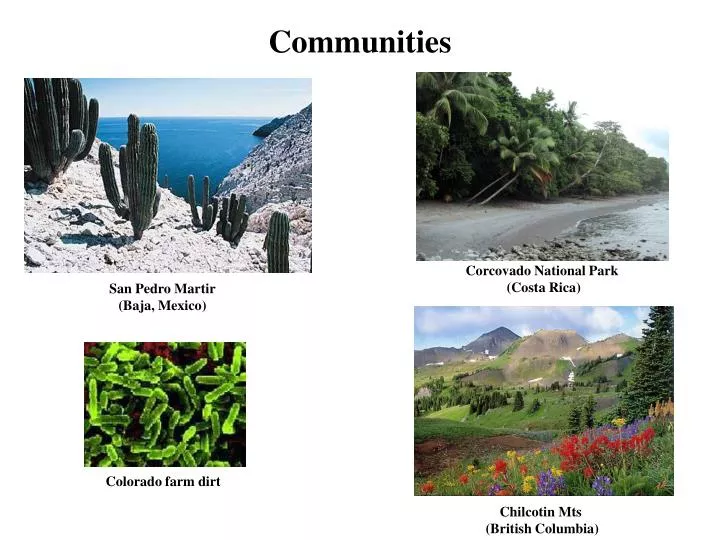
Communities. Corcovado National Park (Costa Rica). San Pedro Martir (Baja, Mexico). Colorado farm dirt. Chilcotin Mts (British Columbia). Communities. Creosote flats — Mojave desert ( Larrea divaricata ). Communities. Venezuelan rainforest (Angel Falls).

E N D
Communities Corcovado National Park (Costa Rica) San Pedro Martir (Baja, Mexico) Colorado farm dirt Chilcotin Mts (British Columbia)
Communities Creosote flats — Mojave desert (Larrea divaricata)
Communities Venezuelan rainforest (Angel Falls)
How can we quantify these differences? • Species richness – The number of species per unit area • Species evenness – The relative abundance of individuals among the species within an area • Species diversity – The combined richness and evenness of species within an area
Species richness • Simply count the number of species within a fixed area Richness = 3 Richness = 1
A problem with species richness • Species richness ignores species evenness Richness = 3 Richness = 3
How can species evenness be incorporated? Species diversity – Measures both species richness and evenness The Shannon Index:
How do you use the Shannon Index? H =-[.333(-1.10) +. 333(-1.10) +. 333(-1.10)] =1.10 H =-[.083(-2.49) +. 083(-2.49) +. 833(-.18)] = 0.56
What does the Shannon Index really tell us? • The greater the value of H the greater the likelihood that the next individual chosen will not belong to the same species as the previous one H = 1.10 H = 0.56
A problem with diversity indices • Two communities with the same diversity index do not necessarily have the same species richness and evenness H Bottom Line: Information is lost when a community is described by a single number!
A graphical solution: rank-abundance curves Step 1: Count the numbers of each species within a defined area
Rank-abundance curves Step 2: Calculate the frequency of each species
Rank-abundance curves Step 3: Plot the species frequencies as a function of frequency rank Frequency or Relative abundance Rank
A general pattern in rank-abundance Tropical wet forest Tropical dry forest Tropical Bats Marine copepods British birds Log scale A consistent result: Coexistence of multiple ecologically similar species
Applying the theory to reserve design (A practice problem) • You are tasked with selecting between three potential locations for a new national park • Your goal is to maximize the long term species richness of passerine birds within the park • Previous research has shown that the birds meet the assumptions of the equilibrium model 12km2 8km2 5km2 5km 4km 3km Mainland source pool: P = 36
Applying the theory to reserve design (A practice problem) Previous research has also shown that: • I = 2/x where x is distance to the mainland • E = .4/A where A is the area of the island • Which of the three potential parks would best preserve passerine bird species richness? 12km2 8km2 5km2 5km 4km 3km Mainland source pool: P = 36
What explains persistence of multiple species? • Multiple ecologically similar species often coexist within communities • Superficially, this is inconsistent with the “competitive exclusion principle” • We know that resources are, at least in some cases limiting • We know that limited resources lead to competition • Lotka-Volterra tells us that ecologically similar species are unlikely to coexist • What forces maintain species diversity within communities?
What explains persistence of multiple species? • Spatio-Temporal variability and the Intermediate Disturbance Theory • Interactions with grazers and predators • Neutral theory
Spatial variability and dispersal are insufficient • Unless dispersal is very high or competition very weak, communities will consist of a single dominant species and many very rare species • This is not what we see in real data
What causes temporal variability? • Disturbance opens up new, unoccupied, habitats
The process of succession: Glacier Bay N.P. • Glaciers have been continually receding • Unoccupied habitat is continually appearing • Process has been studied for the past 80 years • Step 1 • Colonization by mosses, Dryas, and willow • Dryas fixes nitrogen increasing nitrogen content of soil • Step 2 • Colonization by Alnus; Dryas and willow displaced • Alnus species fix nitrogen and acidify the soil • Step 3 • Colonization by Sitka spruce; Alnus displaced • Spruce increases carbon content of soil improving aeration and water retention • Step 4 • Colonization by Hemlock • No further change; Spruce-Hemlock forest persists indefinitely
A model of succession • The resource ratio hypothesis (Tillman, 1988) • Species 1 • Requires minimal nutrient • Requires high light • Species 2 • Requires moderate nutrient • Requires medium-high light • Species 2 • Requires significant nutrient • Requires medium light • Species 2 • Requires abundant nutrient • Requires minimal light Light Nutrient Relative abundance Nutrient or light availability Time
Temporal variability alone is insufficient Light Nutrient Relative abundance Nutrient or light availability • Only several of all possible species generally coexist at any point in time • Species coexistence is transient ultimately one dominant species prevails Time
The intermediate disturbance hypothesis (Connell, 1978) • Assumptions of the IDH • Species differ in their dispersal ability • Pioneer species require few nutrients, high light, and disperse well (r selected) • Late successional species require abundant nutrients, low light, and disperse poorly (k selected) • Repeated disturbances occur (e.g., Fire, logging, landslides, flooding, etc.) Light Nutrient Strong dispersal ability Weak dispersal ability Relative abundance Nutrient or light availability Time
The intermediate disturbance hypothesis (Connell, 1978) If the disturbance rate is too low Light Nutrient Strong dispersal ability Weak dispersal ability Relative abundance Nutrient or light availability • Only a single late successional species remains. All other species extinct. Time
The intermediate disturbance hypothesis (Connell, 1978) If the disturbance rate is too high Light Nutrient Strong dispersal ability Weak dispersal ability Relative abundance Nutrient or light availability • Only a pioneer species remains. All other species extinct. Time
The intermediate disturbance hypothesis (Connell, 1978) If the disturbance rate is intermediate Light Nutrient Strong dispersal ability Weak dispersal ability Relative abundance Nutrient or light availability • All species remain Time
A test of the IDH: Intertidal algal communities (Sousa, 1979) • First studied succession in the absence of disturbance • Studied algal succession on intertidal boulders • Scraped natural rocks clean • Implanted concrete blocks • Found a stereotypical pattern • Steps in algal succession • Initially colonized by the green alga Ulva • Later colonized by four species of red alga • Within 2-3 years each rock or block is a monoculture covered by a single species of red algae
A test of the IDH: Intertidal algal communities (Sousa, 1979) • Next, studied succession in the presence of disturbance • Calculated the wave force needed to roll each boulder at study site • Classified boulders according to force required to move them, an index of “disturbability” • Calculated algal species richness on all boulders • Results • Amount of bare (uncolonized space) decreased with boulder size • confirms that larger boulders were disturbed less • 2. Species richness was greatest on boulders in the intermediate size class • Supports the IDH
Interactions with grazers and predators • Grazing and predation reduce biomass of graze or abundance prey • Can be viewed as a form of disturbance
Grazing and species diversity Zeevalking and Fresco (1977) • Studied impact of rabbit grazing on flora of sand dunes in the Netherlands • Estimated the intensity of rabbit grazing in 1m2 plots located on five different sand dunes • Estimated the species richness in each plot • Grazing increased species richness • Species richness was maximized at intermediate grazing intensities Species richness Grazing pressure
Predation and species diversity Pisaster ochraceus (Ochre star fish) Rocky intertidal — Washington coast
Pisaster are major predators of the intertidal Mytilus californianus (California blue mussel) Balanus glandula (Acorn Barnacle) Pisaster ochraceus (Ochre star fish) Mitella polymerus (Gooseneck barnacle)
Under natural conditions, all 3 prey species occur High tide Low tide
A classic experiment (Paine, 1966) • Established two study plots in the rocky-intertidal zone of Mukkaw • Bay, Washington on June 1963 • In one plot Pisaster was removed • The other plot acted as an unmanipulated control
Species richness actually declined • By September of 1963 Balanus glandula occupied 80% of the available space • By June of 1964 Balanus had been almost completely displaced by Mytilus californianus • In contrast to the plot where Pisaster had been removed, the control plot maintained a steady level of species richness with all three prey species present • These results demonstrate that the predatory starfish, Pisaster, actually maintained prey species richness!
Why did this occur? • Pisaster is a major predator of the three competing intertidal organisms • In the absence of predation by Pisaster the superior competitor excludes all other species (competitive exclusion) • In the presence of Pisaster, however, the density of the best competitor is limited by predation, allowing coexistence • Pisaster acts as a keystone predator, playing a significant role in shaping community structure
Diet switching and frequency dependence • Predators and grazers may actively switch from rare to common prey • Generates negative frequency dependence • Promotes coexistence of multiple prey species Expected if no switching Proportion prey species 1 in diet Expected if no switching Frequency of prey species 1
Diet switching: Zooplanktivorous fish Townsend et al. (1986) • Studied feeding behavior of the roach, Rutilus rutilus, in a small English lake • Fish prefer planktonic waterfleas when available • Switch to sediment dwelling waterfleas when planktonic waterfleas are rare Rutilus rutilus
Neutral theory of biodiversity Hubbell (2001) • Assume that all species are competitively equivalent • In other words, all species within a guild are interchangeable • Assume species have finite population sizes • Under these conditions, the frequency • of species within a habitat changes at • random
Neutral theory of biodiversity Hubbell (2001) • Assume that new species are formed at a fixed rate • Assume that dispersal occurs between habitats • Essentially a model of random genetic drift with mutation and gene flow!!!
Neutral theory of biodiversity Hubbell (2001) • Predictions of this simple model fit the data well • In fact, they fit as well as more complicated models • Yet, we know the assumptions of the model are wrong • Species are not competitively equivalent • Species do exhibit niche differentiation