Download
1 / 74
750 likes | 906 Views
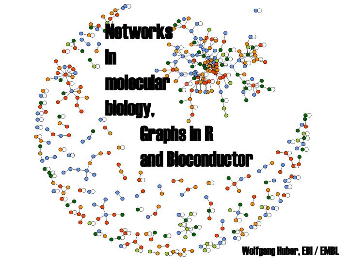
N etworks in m olecular biology , Graphs in R and Bioconductor. Wolfgang Huber, EBI / EMBL. Motivating examples. Regulatory network : components = gene products interactions = regulation of transcription, translation, phosphorylation... Metabolic network:

E N D
Networks in molecularbiology, Graphs in R and Bioconductor Wolfgang Huber, EBI / EMBL
Motivating examples Regulatory network: components = gene products interactions = regulation of transcription, translation, phosphorylation... Metabolic network: components = metabolites, enzymes interactions = chemical reactions Physical interaction network: components = molecules interactions = binding to each other (e.g. complex) Probabilistic network: components = events interactions = conditioning of each other's probabilities Genetic interaction network: components = genes interactions = synthetic, epistatic, … phenotypes
Objectives • Representation of experimental data • a convenient way to represent and visualize experimental data • Map • (visual) tool to navigate through the world of gene products, proteins, domains, etc. • Predictive Model • complete description of causal connections that allows to predict and engineer the behavior of a biological system, like that of an electronic circuit
Definitions Graph := set of nodes + set of edges Edge := pair of nodes Edges can be - directed • undirected • weighted, typed special cases: cycles, acyclic graphs, trees
Network topologies regular all-to-all Random graph (after "tidy" rearrangement of nodes)
Network topologies Scale-free
Random Edge Graphs n nodes, m edges p(i,j) = 1/m with high probability: m < n/2: many disconnected components m > n/2: one giant connected component: size ~ n. (next biggest: size ~ log(n)). degrees of separation: log(n). Erdös and Rényi 1960
Some popular concepts: Small worlds Clustering Degree distribution Motifs
Small world networks Typical path length („degrees of separation“) is short many examples: - communications - epidemiology / infectious diseases - metabolic networks - scientific collaboration networks - WWW - company ownership in Germany - „6 degrees ofKevin Bacon“ But not in - regular networks, random edge graphs
Cliques and clustering coefficient Clique: every node connected to everyone else Clustering coefficient: Random network: E[c]=p Real networks: c » p
Degree distributions p(k) = proportion of nodes that have k edges Random graph: p(k) = Poisson distribution with some parameter l („scale“) Many real networks: p(k) = power law, p(k) ~ k-g „scale-free“ In principle, there could be many other distributions: exponential, normal, …
Growth models for scale free networks Start out with one node and continously add nodes, with preferential attachment to existing nodes, with probability ~ degree of target node. p(k)~k-3 (Simon 1955; Barabási, Albert, Jeong 1999) "The rich get richer" Modifications to obtain g3: Through different rules for adding or rewiring of edges, can tune to obtain any kind of degree distribution
Real networks - tend to have power-law scaling (truncated) - are ‚small worlds‘ (like random networks) - have a high clustering coefficient independent of network size (like lattices and unlike random networks)
Network motifs := pattern that occurs more often than in randomized networks Intended implications duplication: useful building blocks are reused by nature there may be evolutionary pressure for convergence of network architectures
Network motifs Starting point: graph with directed edges Scan for n-node subgraphs (n=3,4) and count number of occurence Compare to randomized networks (randomization preserves in-, out- and in+out- degree of each node, and the frequencies of all (n-1)-subgraphs)
Transcription networks Nodes = transcription factors Directed edge: X regulates transcription of Y
System-size dependence Extensive variable: proportional to system size. E.g. mass, diameter, number of molecules Intensive variable: independent of system size. E.g. temperature, pressure, density, concentration „Vanishing variable“: decreases with system size. E.g. Heat loss through radiation; in a city, probability to bump into one particular person Alon et al.: In real networks, number of occurences of a motif is extensive. In randomized networks, it is non-extensive.
Examples Protein interactions (Yeast-2-Hybrid) Genetic interactions (Rosetta Compendium, Yeast synthetic lethal screen)
promoter Two-hybrid screen Transcription factor activation domain DNA binding domain Idea: „Make potential pairs of interacting proteins a transcription factor for a reporter gene“
Two-hybrid arrays Colony array: each colony expresses a defined pair of proteins
Sensitivity, specificity and reproducibility Specificity – false positives: the experiment reports an interaction even though is really none Sensitivity – false negatives: the experiment reports no interaction even though is really one Problem: what is the objective definition of an interaction? (Un)reproducibility: the experiment reports different results when it is repeated „The molecular reasons for that are not really understood...“ (Uetz 2001)
Rosetta compendium 568 transcript levels 300 mutations or chemical treatments
Transcriptional regulatory networksfrom "genome-wide location analysis" regulator := a transcription factor (TF) or a ligand of a TF tag: c-myc epitope 106 microarrays samples: enriched (tagged-regulator + DNA-promoter) probes: cDNA of all promoter regions spot intensity ~ affinity of a promotor to a certain regulator
Transcriptional regulatory networksbipartite graph 106 regulators (TFs) regulators 6270 promoter regions promoters
Global Mapping of the Yeast Genetic Interaction Network Amy Hin Yan Tong,…49 other people, …Charles Boone Science 303 (6 Feb 2004)
Buffering and Genetic Variation In yeast, ~73% of gene deletions are "non-essential" (Glaever et al. Nature 418 (2002) In Drosophila, ~95% (Boutros et al. Science 303 (2004)) In Human, ca. 1 SNP / 1.5kB Evolutionary pressure for robustness Bilateral asymmetry is positively correlated with inbreeding Most genetic variation is neutral to fitness, but may well affect quality of life Probably mechanistic overlap between buffering of genetic, environmental and stochastic perturbations
Models for Buffering Comparison of single mutants to double mutants in otherwise isogenic genetic background Synthetic Genetic Array (SGA) analysis (Tong, Science 2001): cross mutation in a "query" gene into a (genome-wide) array of viable mutants, and score for phenotype. Tong 2004: 132 queries x 4700 mutants
Buffering A buffered by B (i) molecular function of A can also be performed by B with sufficient efficiency (ii) A and B part of a complex, with loss of A or B alone, complex can still function, but not with loss of both (iii) A and B are in separate pathways, which can substitute each other's functions. structural similarity - physically interaction - maybe, but neither is necessary.
Selection of 132 queries o actin-based cell polarity o cell wall biosynthesis o microtubule-based chromosome segregation o DNA synthesis and repair Reproducibility Each screen 3 times: 3x132x4700 = 1.8 Mio measurements 25% of interactions observed only 1/3 times 4000 interactions amongst 1000 genes confirmed by tetrad or random spore analysis ("FP neglible") FN rate: 17-41%
Statistics Hits per query gene: range 1...146, average 34 (!) power-law (g=-2) Physical interactions: ~8 Dubious calculation: ~100,000 interactions
GO Genes with same or "similar" GO category are more likely to interact
Patterns SGI more likely between genes - withsame mutant phenotype - withsame localization - in same complex (but this explains only 1 % of IAs) - that are homologous (but this explains only 2% of IAs) Genes that have many common SGI partners tend to also physically interact: 30 / 4039 SGI pairs are also physically interacting 27 / 333 gene pairs with >=16 common SGI partners factor: 11
Genetic interaction network SGI more likely between genes - withsame mutant phenotype - withsame localization - in same complex (but this explains only 1 % of IAs) - that are homologous (but this explains only 2% of IAs) A dense small world: Average path-length 3.3 (like random graph) High clustering coefficient (immediate SGI partners of a gene tend to also interact)
Literature Exploring complex networks, Steven H Strogatz, Nature 410, 268 (2001) Network Motifs: Simple Building Blocks of Complex Networks, R. Milo et al., Science 298, 824-827 (2002) Two-hybrid arrays, P. Uetz, Current Opinion in Chemical Biology 6, 57-62 (2001) Transcriptional Regulatory Networks in Saccharomyces Cerevisiae, TI Lee et al., Science 298, 799-804 (2002) Functional organization of the yeast proteome by systematic analysis of protein complexes, AC Gavin et al., Nature 415, 141 (2002) Functional discovery via a compendium of expression profiles, TR Hughes et al., Cell 102, 109-126 (2000) Global Mapping of the Yeast Genetic Interaction Network, AHY Tong et al., Science 303 (2004)
graph, RBGL, Rgraphviz graph basic class definitions and functionality RBGL interface to graph algorithms (e.g. shortest path, connectivity) Rgraphviz rendering functionality Different layout algorithms. Node plotting, line type, color etc. can be controlled by the user.
Creating our first graph library(graph); library(Rgraphviz) edges <- list(a=list(edges=2:3), b=list(edges=2:3), c=list(edges=c(2,4)), d=list(edges=1)) g <- new("graphNEL", nodes=letters[1:4], edgeL=edges, edgemode="directed") plot(g)
Querying nodes, edges, degree > nodes(g) [1] "a" "b" "c" "d" > edges(g) $a [1] "b" "c" $b [1] "b" "c" $c [1] "b" "d" $d [1] "a" > degree(g) $inDegree a b c d 1 3 2 1 $outDegree a b c d 2 2 2 1
Adjacent and accessible nodes > adj(g, c("b", "c")) $b [1] "b" "c" $c [1] "b" "d" > acc(g, c("b", "c")) $b a c d 3 1 2 $c a b d 2 1 1
Undirected graphs, subgraphs, boundary graph • > ug <- ugraph(g) > plot(ug) > sg <- subGraph(c("a", "b", "c", "f"), ug) > plot(sg) > boundary(sg, ug) > $a >[1] "d" > $b > character(0) > $c >[1] "d" > $f >[1] "e" "g"