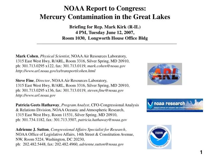
NOAA Report to Congress: Mercury Contamination in the Great Lakes

1. NOAA Report to Congress: Mercury Contamination in the Great Lakes Briefing for Rep. Mark Kirk (R-IL) 4 PM, Tuesday June 12, 2007, Room 1030, Longworth House Office Bldg Mark Cohen, Physical Scientist, NOAA Air Resources Laboratory, 1315 East West Hwy, R/ARL, Room 3316, Silver Spring, MD 20910, ph: 301.713.0295 x122, fax: 301.713.0119, mark.cohen@noaa.gov http://www.arl.noaa.gov/ss/transport/cohen.html Steve Fine, Director, NOAA Air Resources Laboratory, 1315 East West Hwy, R/ARL, Room 3316, Silver Spring, MD 20910, ph: 301.713.0295 x136, fax: 301.713.0119, steven.fine@noaa.gov http://www.arl.noaa.gov Patricia Geets Hathaway, Program Analyst, CFO-Congressional Analysis & Relations Division, NOAA Oceanic and Atmospheric Research, 1315 East West Hwy, Room 11531, Silver Spring, MD 20910, ph: 301.734.1182, fax: 301.713.3507, patricia.hathaway@noaa.gov Adrienne J. Sutton, Congressional Affairs Specialist for Research, NOAA Office of Legislative Affairs, 14th Street & Constitution Avenue, NW, Room 5224, Washington, DC 20230, ph: 202.482.5448, fax: 202.482.4960, adrienne.sutton@noaa.gov 1

2. NOAA Report to Congress on Mercury Contamination in the Great Lakes http://www.arl.noaa.gov/data/web/reports/cohen/NOAA_GL_Hg.pdf • The Conference Report accompanying the consolidated Appropriations Act, 2005 (H. Rpt. 108-792) requested that NOAA, in consultation with the EPA, report to Congress on mercury contamination in the Great Lakes, with trend and source analysis. • Reviewed by NOAA, EPA, DOC, White House Office of Science and Technology Policy, and Office of Management and Budget (OMB); • Preparation / review process took more than 2 years. • Transmitted to Congress on May 14, 2007 2

3. (this page intentionally left blank)

4. The Atmospheric Transport and Deposition of Mercury to the Great Lakes • A. Introduction • B.Atmospheric Emissions • C.Overview of Atmospheric Mercury Modeling • D.Illustrative Modeling Results for a Single Source • E.Overall Modeling Methodology • F.Model Uncertainties • 1)Emissions • 2)Atmospheric Phase Behavior • 3)Atmospheric Chemistry • 4)Wet and Dry Deposition • 5)Meteorological Data • G.Model Evaluation • H.Atmospheric Modeling Results • 1)Lake Michigan • 2)Lake Superior • 3)Lake Huron • 4)Lake Erie • 5)Lake Ontario • 6)Combined Great Lakes • I.Potential Next Steps • J.Summary of Great Lakes Atmospheric Mercury Deposition This report does not attempt to report on all of the many aspects of mercury contamination in the Great Lakes. It is limited to the following two primary components: • Analysis of the atmospheric transport and deposition of U.S. and Canadian anthropogenic mercury emissions to the Great Lakes using the NOAA HYSPLIT-Hg model; • Illustrative literature data regarding trends in Great Lakes mercury contamination. • Trends in Great Lakes Mercury • A. Mercury Emissions • B. Mercury Deposition • 1) Wet deposition measurements in the Great Lakes region • 2) Other mercury wet deposition measurements • 3) Modeled deposition to the Great Lakes from U.S. and Canadian sources • C. Mercury Concentrations in Sediments • D. Mercury Concentrations in Biota • E. Summary of Great Lakes Mercury Trend Data 4

5. 5

6. 6

7. 7

8. Key Findings • Source-attribution information is needed for policy development • Atmospheric modeling is the only way to obtain comprehensive source-attribution information • Monitoring alone provides values/trends at a few locations, but it cannot answer certain key questions • Why are the values what they are, e.g., source attribution? • What are the values in other locations? Why are there (or are there not) spatial and/or temporal trends? • What might happen in the future under different environment/policy conditions? • However, atmospheric monitoring data are essential to evaluate and improve models • Atmospheric mercury modeling and monitoring are far more useful together than they are apart • Monitoring programs need to be designed with model evaluation and improvement in mind • The fate and transport of atmospheric mercury is complex • Scarcity of modeling resources and monitoring* & process** data means that models haven’t been adequately evaluated • * monitoring data refers to atmospheric concentration measurements in air and precipitation • ** process data refers to measurements of fundamental phenomena such as chemical reactions and atmospheric deposition processes • Thus, while there are many uncertainties in current models, the magnitude of the uncertainties is poorly known • A number of steps could be taken to characterize uncertainties and reduce them if necessary • Collection of additional monitoring data and carrying out process research • Increased quality and frequency of emissions data and inventories • Comprehensive model evaluation/improvement, sensitivity analyses, and intercomparison experiments • Modeling has provided preliminary, useful information about mercury deposition to the Great Lakes • Detailed, source-attribution results for U.S. and Canadian anthropogenic sources • Of these sources, the biggest contribution is from U.S. coal-fired power plants in the Great Lakes region • Waste incineration emissions and deposition decreased significantly during the 1990’s, but timing poorly known • Further work could provide more complete information • Characterize/reduce uncertainties as described above • Extend model to include global anthropogenic and natural sources • Carry out simulations of past, present, and potential future atmospheric deposition and source-attribution • Trend data have been assembled for mercury in Great Lakes sediments, biota, emissions and deposition • Levels tended to rise from ~1900 through the 1960’s and 1970’s, with a peak during WWII. • Reductions in the ~1970’s, possibly due to the closure or changes at regional mercury-based chlor-alkali factories • Levels have remained relatively constant since the 1980’s • Interpretation of trend data is complicated by a scarcity of data on historical emissions and loading rates 8

9. Atmospheric Models ? Air Concentration Network Mercury Deposition Network (MDN) (wet deposition only) Emissions Inventories Understanding and Decisions • To evaluate and improve atmospheric models, emissions inventories must be: • Accurate for each individual source (especially for large sources), including variations • For the same time periods as measurements used for evaluation • For all forms of mercury Deposition For Entire Region ? Inputs for Ecosystem Models Atmospheric Monitoring Understanding Trends ? ? • To evaluate and improve atmospheric models, atmospheric monitoring must be: • For air concentrations (not just wet deposition) • For all forms of mercury • For sites impacted by sources (not just background sites) • At elevations in the atmosphere (not just at ground level) Source-attribution; Scenarios Incin Manuf Fuel (not coal electric) Coal-electric Coal Scenarios (slide 8) Hg Dep to Lake Michigan (g/km2-yr)

10. Why do we need atmospheric mercury models? • to get comprehensive source attribution information ...we don’t just want to know how much is depositing at any given location, we also want to know where it came from: • different source regions (local, regional, national, continental, global) • different jurisdictions (different states and provinces) • anthropogenic vs. natural emissions • different anthropogenic source types (power plants, waste incin., etc) • to estimate deposition over large regions …because deposition fields are highly spatially variable, and one can’t measure everywhere all the time… • to estimate dry deposition ... presently, dry deposition can only be estimated via models • to evaluate potential consequences of alternative future emissions scenarios 10

11. HYSPLIT-Hg Atmospheric Fate and Transport Model Hg(0) Hg(0) from distant sources atmospheric chemistry interconverts mercury forms Hg(II) Hg(p) atmospheric emissions of Hg(0), Hg(II), Hg(p) Where does the mercury come from that is depositing to any given waterbody or watershed? atmospheric deposition to the watershed atmospheric deposition to the water surface • How much from local/regional sources? • How much from global sources? • Monitoring alone cannot give us the answer • atmospheric models required, “ground-truthed” by atmospheric monitoring Humans and wildlife affected primarily by eating fish containing mercury Best documented impacts are on the developing fetus: impaired motor and cognitive skills Mercury transforms into methylmercury in soils and water, then canbioaccumulate in fish 11 adapted from slides prepared by USEPA and NOAA

12. Challenges / critical data needs for model evaluation: • Need wet deposition – like data collected in the existing Mercury Deposition Network (MDN) -- but also need ambient air concentrations of different forms of mercury, i.e., reactive gaseous mercury [RGM], particulate mercury [Hg(p)], and elemental mercury [Hg(0)]. Ambient air concentration data is extremely scarce. • Need sites that are impacted by large sources as well as background sites that are not impacted by large sources. Most current measurement sites are “background” sites. • Most current measurements are currently done at ground level. Also needed are measurements in the atmosphere above the surface (e.g., taken on aircraft, towers…) • Unlike the wet deposition data assembled in the Mercury Deposition Network, for ambient concentration data, there are significant data availability issues for what little such data that there is. • NOAA is playing a central role with EPA in the emerging national mercury ambient concentration measurement network under the umbrella of the National Atmospheric Deposition Program (NADP). NOAA has “donated” the first three sites for this new network. Contingent upon the cooperation of scientists and other agencies, additional sites will be added and this network will be successfully implemented. 12

13. atmospheric chemistry inter-converts mercury forms Hg(0) Hg from other sources: local, regional & more distant Hg(II) Hg(p) atmospheric deposition to the water surface emissions of Hg(0), Hg(II), Hg(p) atmospheric deposition to the watershed Measurement of ambient air concentrations Measurement of wet deposition WET DEPOSITION • complex – hard to diagnose • weekly – many events • background – but also need monitoring sites near sources AMBIENT AIR CONCENTRATIONS • more fundamental – easier to diagnose • need continuous – episodic source impacts • need different forms of mercury – at least RGM, Hg(p), Hg(0) • need data at surface and above 13

14. Figure 12. Largest sources of total mercury emissions to the air in the U.S. and Canada. As discussed in the text, the data generally represent emissions for 1999-2000. 14

15. Canaan Valley Institute-NOAA Beltsville EPA-NOAA Grand Bay NOAA Largest sources of total mercury emissions to the air in the U.S. and Canada, based on the U.S. EPA 1999 National Emissions Inventory and 1995-2000 data from Environment Canada Three NOAA sites committed to emerging inter-agency speciated mercury ambient concentration measurement network (comparable to Mercury Deposition Network (MDN) for wet deposition, but for air concentrations) 15

16. Monitoring Site NOAA SEARCH USGS UWF/FSU MDN type of mercury emissions source coal-fired power plant total atmospheric mercury emissions (kg/yr, 1999 EPA NEI) waste incinerator manufacturing 1 – 50 metallurgical 50 - 100 other fuel combustion 100 - 200 200 - 400 Location of the new NOAA Grand Bay NERR Atmospheric Mercury monitoring site, other atmospheric Hg monitoring sites, and major Hg point sources in the region (according to the EPA 1999 NEI emissions inventory) Mississippi Alabama Barry paper manuf paper manuf AL02 Pascagoula MSW incin Mobile Molino Crist Victor J. Daniel Holcim Cement Pace OLF haz waste incin Ellyson AL24 Weeks Bay Mobile Bay Jack Watson Pascagoula NOAA Grand Bay NERR Hg site 16

17. Monitoring sites rural AQS other AQS NADP/MDN CASTNet Symbol color indicates type of mercury source Hg site IMPROVE coal incinerator metals manuf/other Symbol size and shape indicates 1999 mercury emissions, kg/yr 1 - 50 50 - 100 100 - 200 200 – 400 400 - 700 700 – 1000 > 1000 Location of the new NOAA-EPA Atmospheric Mercury monitoring site at Beltsville Maryland, other atmospheric monitoring sites, and major Hg point sources in the region (according to the EPA 1999 NEI emissions inventory) Beltsville monitoring site Brunner Island Large Incinerators: 3 medical waste, 1 MSW, 1 haz waste (Total Hg ~ 500 kg/yr) Harford County MSW Incin Brandon Shores and H.A. Wagner 100 miles from DC Montgomery County MSW Incin Eddystone Dickerson Arlington - Pentagon MSW Incin Possum Point the region between the 20 km and 60 km radius circles displayed around the monitoring site might be considered the “ideal” location for sources to be investigated by the site Chalk Point Morgantown Bremo 17

18. Emissions inventories are fundamental inputs for atmospheric mercury models. • Accurate inventories are required for model evaluation and improvement, as well as for accurate simulations once the models are “perfected” Inventories need to be improved • Inventories need to be more complete; more accurate; more transparent; uncertainties estimated. • Emissions estimates needed for all forms of mercury [RGM, Hg(p), Hg(0)]. Long delay before inventories released • 2002 U.S. inventory released in 2007; till now, latest available inventory was for 1999. • Can’t use new measurement data to evaluate models if the inventories aren’t available. Inventories must be prepared more frequently • Currently, the only available source-by-source inventories for the U.S. are for 1999 and for 2002. • Large emissions reduction between ~1990 and ~2000, but not known when reductions occurred at individual facilities. Thus, very difficult to interpret trends in monitoring data. Inventories need to include information about major “step-change” events • There can be abrupt “step-changes” in emissions due to shutdowns, maintenance, closures, installation of new pollution control devices, feedstock changes, and process changes, etc. • Currently, the only data available in emissions inventories is an annual average. Therefore, it is difficult to interpret variations/trends in ambient measurements. Data are needed on short-term variations on time scales of minutes to hours • There are short-term variations in emissions, on scales of minutes to hours. We need to know about these short term variations to correlate emissions with measurements. • Clean Air Mercury Rule requires ~weekly total-Hg measurements for coal-fired power plants. Continuous Emissions Monitors (CEM’s) needed – and not just on coal-fired power plants. • CEM’s must measure different forms of mercury or will not be useful in developing source-receptor info. 18

19. 2000 Global Inventory New York inventory 1995 Canada Inventory 2000 Canada Inventory Ontario inventory ? 1999 US Inventory 2002 US Inventory ? speciated atmospheric Hg measurements at site x Hypothetical – just for illustration purposes speciated atmospheric Hg measurements at site y speciated atmospheric Hg measurements at site z For model evaluation, inventory must be accurate and for same period as measurements (a big challenge!) 95 96 97 98 99 00 01 02 03 04 05 06 07 08 09 10 11 12 13 14 15 19

20. Importance of time-resolved, speciated emissions measurements • Based on CEM data collected at coal-fired power plants, it appears that there can be significant variations in emissions of Hg(2), Hg(0) and Hg(p) over time scales of minutes to hours • Meteorological conditions – and hence source-receptor relations – can vary significantly over time scales of minutes to hours. • If we are collecting speciated ambient concentration data downwind of sources on time scales of minutes to hours, and the source emissions are varying on the same time scales, it is critical to have data regarding the emissions variations. Without it, severe limitations on what can be learned from the ambient concentration data. • Speciated Continuous Emissions Monitors (CEM’s) are commercially available. • CAMR does not appear to require speciated emissions data, and does not appear to require time-resolved data on the order of minutes to hours (i.e., longer term data are all that is required, e.g., on the order of ~1 week). So, we have a problem. • For the purposes of model evaluation and improvement, and to the extent possible, it would be helpful if speciated, time-resolved CEM’s could be installed at large Hg sources significantly impacting critical model-evaluation monitoring sites. 20

21. Hg from other sources: local, regional & more distant atmospheric deposition to the water surface atmospheric deposition to the watershed Measurement of ambient air concentrations Measurement of wet deposition 21

22. 22

23. Figure 44. Largest modeled contributors to Lake Michigan (close-up). (same legend as previous slide) 23

24. Atmospheric Deposition Flux to Lake Michigan from Anthropogenic Mercury Emissions Sources in the U.S. and Canada 24

25. Top 25 modeled sources of atmospheric mercury to Lake Michigan (based on 1999 anthropogenic emissions in the U.S. and Canada) 25

26. Emissions and deposition to Lake Michigan arising from different distance ranges (based on 1999 anthropogenic emissions in the U.S. and Canada) … but these “local” emissions are responsible for a large fraction of the modeled atmospheric deposition Only a small fraction of U.S. and Canadian emissions are emitted within 100 km of Lake Michigan… 26

27. Next Steps: As resources permit, steps could be taken to refine/extend mercury modeling, e.g.: Extension of the model from North American domain to simulate impacts of global sources Inclusion of the impact of natural emissions and re-emissions of anthropogenic mercury. The use of more detailed meteorological data (e.g., described on finer spatial scales). Development of a system for incorporating observed precipitation data into the model. Further evaluation of the model against wet deposition data and ambient concentration data for elemental, ionic, and particulate mercury. Process-related measurements of atmospheric chemistry, phase-partitioning behavior, and atmospheric deposition to evaluate and refine model algorithms. Sensitivity tests -- investigating the influence of uncertainties in model inputs and model algorithms -- to help determine which uncertainties are the most critical for model improvement. Linkage of the atmospheric model to other models to form a multi-media mercury modeling system to track mercury from emissions to ecosystem loading to food chain bioaccumulation to human exposure. Use of updated emissions inventories as inputs to the model. Estimation of the time-course of atmospheric loading to the Great Lakes by running the model over long periods using a continuous record of historical emissions. Estimation of the impacts of potential future emissions scenarios. Participation in additional model comparison studies. 27

28. Relative Importance of Anthropogenic vs. Natural Sources? • Many studies have shown increased amounts of bio-available mercury in ecosystems due to anthropogenic activities (~2x – 5x, sometimes more), but a large number of factors influence the relative increases, e.g., proximity to sources, relative proportions of different forms of mercury emitted from sources, particular biogeochemistry of the ecosystem, etc. • Relative Importance of Global vs. Domestic Sources? • NOAA HYSPLIT-Hg work to date has not yet attempted to explicitly answer this question. • New work could be done to address this issue. • It is noted, however, that in many cases, much of the deposition in U.S. regions with significant sources appears like it can be accounted for by consideration of U.S sources alone. • A few estimates have been made using other models. Results to date suggest that: • There is no “one” answer – the relative importance varies from location to location. • In regions with significant sources, the relative importance of global sources appears to be diminished • The answer also obviously varies depending on the time period • Like with analysis of national sources, the global modeling to date is limited by a number of uncertainties (emissions inventories, atmospheric chemistry, deposition processes) and the evaluation of the models is significantly limited by a lack of observations. Thus, the significance of the uncertainties is not well known. 28

29. Figure 40. WI99, 72-hour back trajectories for high deposition event during the week of 4/18/00 to 4/25/00. Butler, T., Likens, G., Cohen, M., Vermeylen, F. (2007). Mercury in the Environment and Patterns of Mercury Deposition from the NADP/MDN Mercury Deposition Network. Final Report to USEPA. 29 http://www.arl.noaa.gov/data/web/reports/cohen/51_camd_report.pdf

30. Summary of Great Lakes Region Trend Information for Atmospheric Mercury Emissions and Deposition • Trends in Great Lakes region atmospheric mercury emissions: • Data are scarce and uncertain, but it appears that they rose significantly from ~1880 until ~1945, were approximately level from 1945-1970, and decreased between 1970-1980. • Trends in U.S. atmospheric mercury emissions from the early 1990’s to ~2001: • Significant decrease in emissions from municipal and medical waste incinerators, but exact timing of changes at individual facilities poorly characterized. • Emissions from coal-fired electricity generation and other source categories were relatively constant. • Trends in Canadian atmospheric mercury emissions: • From 1990-2000, Canadian emissions are reported to have decreased by ~75 percent, largely due to process changes at metal smelting facilities. • Trends in mercury wet deposition at monitoring sites in the Great Lakes region: • Five long-term Mercury Deposition Network sites, with data beginning in 1996. • For this report, data for 1996-2003 examined. • Possible decrease between 2000 and 2001, and this may have been related to decreases in regional mercury emissions from waste incinerators. • There were only moderate changes in estimated ionic mercury emissions in the vicinity of these sites between 1995-1996 and 1999-2001, but the precise timing of these changes is not known. Thus, it is difficult to determine if the trends in precipitation mercury concentrations are related to these reductions. • Trends in mercury deposition to the Great Lakes: • Trends in model-estimated deposition to the Great Lakes decreased significantly between 1995-1996 and 1999-2001, primarily due to decreases in emissions from U.S. municipal and medical waste incinerators. • In both periods, the model results suggest that U.S. sources contributed much more to Great Lakes atmospheric mercury deposition than Canadian sources. 30

31. Figure 75. Mercury emissions in North America and the Great Lakes region (1800-1990). • Atmospheric mercury emissions from (a) gold and silver mining in North America; (b) modern anthropogenic sources in North America; and (c) modern anthropogenic sources in the Great Lakes region (including the 8 Great Lakes U.S. states and the province of Ontario). [a reproduction of Figure 2 from Pirrone et al. (1998).] • Pirrone, N., Allegrini, I., Keeler, G., Nriagu, J., Rossman, R., Robbins, J. (1998). Historical atmospheric mercury emissions and depositions in North America compared to mercury accumulations in sedimentary records. Atmos. Environ. 32(5): 929-940. 31

32. Figure 76. Mercury emissions trend data from the U.S. EPA. 32

33. Modeled mercury deposition (kg/year) to the Great Lakes (1995-1996 vs. 1999-2000), arising from anthropogenic mercury air emissions sources in the U.S. and Canada • Model results for atmospheric deposition show that: • U.S. contributes much • more than Canada • Significant decrease • between 1996 and 1999 (primarily due to decreased emissions from waste incineration) Modeled mercury flux (ug/m2-yr) to the Great Lakes (1995-1996 vs. 1999-2000), arising from anthropogenic mercury air emissions sources in the U.S. and Canada 33

34. Figure 77. Great Lakes MDN sites with the longest measurement record. 34

35. Figures 78-83. Mercury concentration in precipitation at long-term MDN sites in the Great Lakes region. 35

36. Summary of Great Lakes Region Trend Information for Sediments and Biota • Trends in mercury in Great Lakes sediments: • Examples of sediment mercury trend data were found for each of the Great Lakes except for Lake Huron. • The data typically show a 1940-1960 peak in sediment mercury, and in some cases there are also secondary peaks in the 1970’s. • Since the 1970’s sediment mercury concentrations appear to have generally been decreasing in the Great Lakes. • . • Trends in mercury levels in Great Lakes biota: • Data on mercury levels in Great Lakes fish and Herring Gull eggs are generally available starting in the 1970’s, while data on levels in mussels are available beginning in 1992. • While there are variations among species and among lakes, the data generally seem to show a reduction from 1970 to the mid-1980’s, with little change since the mid-1980’s. • This is most likely due to the significant reduction that occurred in the 1970’s in effluent discharges to the Great Lakes (and their tributaries) from a number of sources (e.g., chlor-alkali plants). 36

37. Figure 95. Trend in sediment mercury in Lake Michigan. Profile of total mercury (ug/g dry weight) levels in a core sample from Lake Michigan. Source: Marvin, C.; Painter, S., and Rossmann, R. (2004). Spatial and temporal patterns in mercury contamination in sediments of the Laurentian Great Lakes. Env. Research 95(3):351-362. 37

38. Figure 106. Trends in Herring Gull Egg Hg concentrations. Source of data – Canadian Wildlife Service. Total mercury concentrations in eggs from colonies in the Great Lakes region expressed in units of ug Hg/g (wet weight). From 1971 – 1985, analysis was generally conducted on individual eggs (~10) from a given colony, and the standard deviation in concentrations is shown on the graphs. From 1986 to the present, analysis was generally conducted on a composite sample for a given colony. The trend lines shown are for illustration purposes only; they were created by fitting the data to a function of the form y = cxb. 38

39. Figure 107. Mercury concentration in Great Lakes region mussels (1992-2004). Total mercury in mussels (ug/g, on a dry weight basis). In a few cases (e.g. for several sites in 2003), mercury concentrations were below the detection limit. In these cases the concentrations are shown with a white cross-hatched bar at a value of one-half the detection limit; in reality, the mercury concentration could have been anywhere between zero and the detection limit. Source of data: NOAA Center for Coastal Monitoring and Assessment (CCMA) (2006) and “Monitoring Data - Mussel Watch” website: http://www8.nos.noaa.gov/cit/nsandt/download/mw_monitoring.aspx 39

40. Figure 101. Mercury concentration trends Great Lakes Walleye. Total mercury concentrations (ppm or ug Hg/g). Sources of data: Ontario Ministry of the Environment (2006b), for 45-cm Walleye data, and Environment Canada (2006), for data on Lake Erie Walleye ages 4-6. 40

41. Figure 102. Total mercury levels in Great Lakes Rainbow Smelt, 1977-2004. Source of data: Environment Canada (2006). Note that the scales for the lakes are different. 41

42. Model-estimated U.S. utility atmospheric mercury deposition contribution to the Great Lakes: HYSPLIT-Hg (1996 meteorology, 1999 emissions) vs. CMAQ-Hg (2001 meteorology, 2001 emissions). Note: Uncertainty estimates for these results could be developed in future work 42

43. Model-estimated U.S. utility atmospheric mercury deposition contribution to the Great Lakes: HYSPLIT-Hg (1996 meteorology, 1999 emissions) vs. CMAQ-Hg (2001 meteorology, 2001 emissions). • This figure also shows an added component of the CMAQ-Hg estimates -- corresponding to 25% of the CMAQ-Hg results – in an attempt to adjust the CMAQ-Hg results to account for the deposition underprediction found in the CMAQ-Hg model evaluation. Note: Uncertainty estimates for these results could be developed in future work 43 43

44. HYSPLIT 1996 Different Time Periods and Locations, but Similar Results ISC: 1990-1994 44

45. Total Gaseous Mercury (ng/m3) at Neuglobsow: June 26 – July 6, 1995 45

46. Total Particulate Mercury (pg/m3) at Neuglobsow, Nov 1-14, 1999 46

47. EMEP Intercomparison Study of Numerical Models for Long-Range Atmospheric Transport of Mercury Intro-duction Stage I Stage II Stage III Conclu-sions Chemistry Hg0 Hg(p) RGM Wet Dep Dry Dep Budgets Reactive Gaseous Mercury at Neuglobsow, Nov 1-14, 1999 47

48. Ryaboshapko, A., et al. (2007). Intercomparison study of atmospheric mercury models: 1. Comparison of models with short-term measurements. Science of the Total Environment376: 228–240. http://www.arl.noaa.gov/data/web/reports/cohen/49_EMEP_paper_2.pdf 48

49. Ryaboshapko, A., et al. (2007). Intercomparison study of atmospheric mercury models: 2. Modelling results vs. long-term observations and comparison of country deposition budgets. Science of the Total Environment 377: 319-333. http://www.arl.noaa.gov/data/web/reports/cohen/49_EMEP_paper_2.pdf 49

50. Lagrangian Puff Atmospheric Fate and Transport Model 0 1 2 TIME (hours) The puff’s mass, size, and location are continuously tracked… = mass of pollutant (changes due to chemical transformations and deposition that occur at each time step) Phase partitioning and chemical transformations of pollutants within the puff are estimated at each time step Initial puff location is at source, with mass depending on emissions rate Centerline of puff motion determined by wind direction and velocity Dry and wet deposition of the pollutants in the puff are estimated at each time step. deposition 2 deposition to receptor deposition 1 lake NOAA HYSPLIT MODEL 50