Figure 2: AMSR-E 12.5 km Ice Concentration

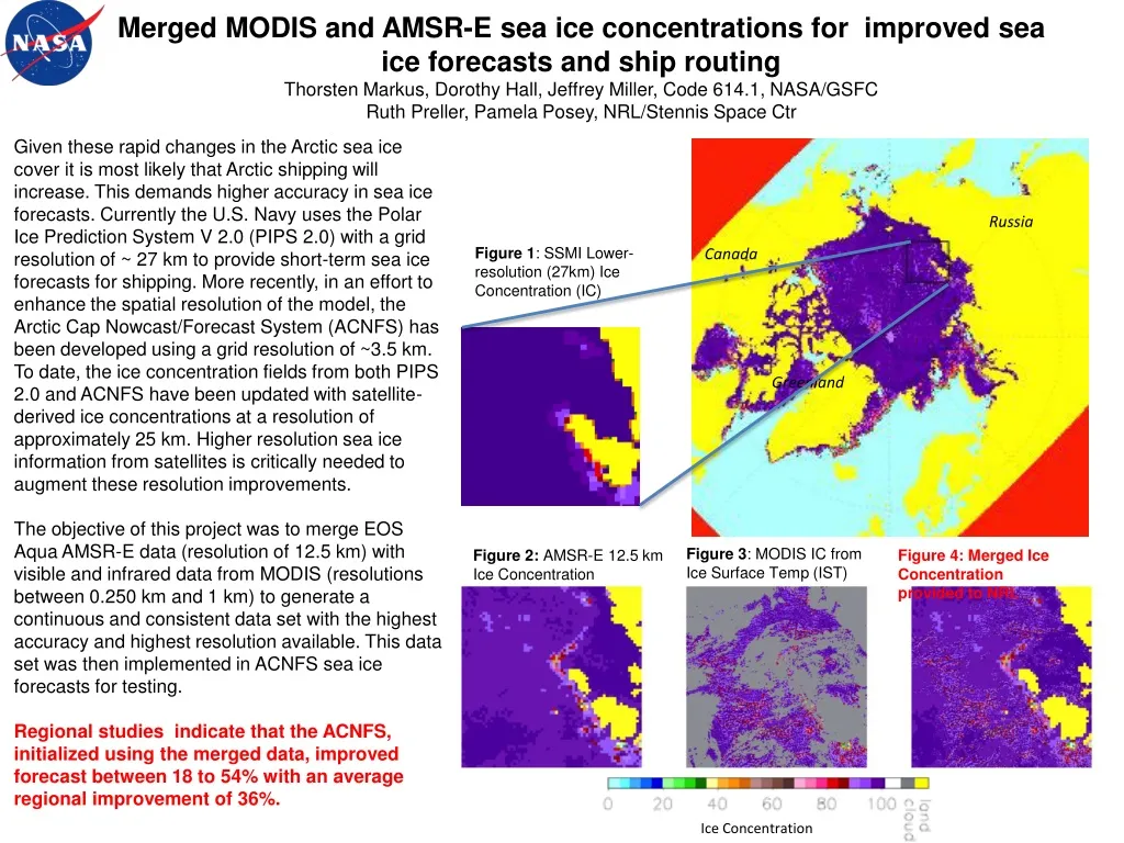
1. Merged MODIS and AMSR-E sea ice concentrations for improved sea ice forecasts and ship routing Thorsten Markus, Dorothy Hall, Jeffrey Miller, Code 614.1, NASA/GSFC Ruth Preller, Pamela Posey, NRL/Stennis Space Ctr Given these rapid changes in the Arctic sea ice cover it is most likely that Arctic shipping will increase. This demands higher accuracy in sea ice forecasts. Currently the U.S. Navy uses the Polar Ice Prediction System V 2.0 (PIPS 2.0) with a grid resolution of ~ 27 km to provide short-term sea ice forecasts for shipping. More recently, in an effort to enhance the spatial resolution of the model, the Arctic Cap Nowcast/Forecast System (ACNFS) has been developed using a grid resolution of ~3.5 km. To date, the ice concentration fields from both PIPS 2.0 and ACNFS have been updated with satellite-derived ice concentrations at a resolution of approximately 25 km. Higher resolution sea ice information from satellites is critically needed to augment these resolution improvements. The objective of this project was to merge EOS Aqua AMSR-E data (resolution of 12.5 km) with visible and infrared data from MODIS (resolutions between 0.250 km and 1 km) to generate a continuous and consistent data set with the highest accuracy and highest resolution available. This data set was then implemented in ACNFS sea ice forecasts for testing. Regional studies indicate that the ACNFS, initialized using the merged data, improved forecast between 18 to 54% with an average regional improvement of 36%. Russia Canada Figure 1: SSMI Lower-resolution (27km) Ice Concentration (IC) Greenland Figure 3: MODIS IC from Ice Surface Temp (IST) Figure 2: AMSR-E 12.5 km Ice Concentration Figure 4: Merged Ice Concentration provided to NRL Ice Concentration

2. Investigators: Thorsten Markus, Dorothy Hall, Jeffrey Miller NASA/GSFC • Ruth Preller, Pamela Posey, Naval Research Laboratory, Stennis Space Center • E-mail: Thorsten.Markus@nasa.gov • Phone: 301-614-5882 • References: • Markus, T., D.K. Hall, J. Miller, P. Posey, R. Preller • Merged EOS Aqua/Terra MODIS and AMSR-E sea ice information for improved sea ice forecasts and ship routing • NASA Applied Sciences Program, FEASIBILITY, Final Report, 2010. • Data Sources: • Cavalieri, Donald, Thorsten Markus, and JosefinoComiso. 2004, updated daily. AMSR-E/Aqua Daily L3 12.5 km Brightness Temperature, Sea Ice Concentration, & Snow Depth Polar Grids V002, 2008-06-01 to 2008-06-30. Boulder, Colorado USA: National Snow and Ice Data Center. Digital media • Hall, Dorothy K., George A. Riggs, and Vincent V. Salomonson. 2007, updated daily. MODIS/Aqua Sea Ice Extent and IST Daily L3 Global 4km EASE-Grid Day V005, 2008-06-01 to 2008-06-30. Boulder, Colorado USA: National Snow and Ice Data Center. Digital media. • Technical Description of Image: Sea ice concentration in the East Siberian Sea showing • (Figure 1) ice concentration from SSM/I at 27km as currently used in the forecast system • (Figure 2) 12.5 km sea ice concentration from AMSR-E • (Figure 3) 4km sea ice concentration derived from the MODIS ice surface temperature (clouds are gray); ice • concentrations are derived in a way that ensures consistency between the AMSR-E and MODIS • retrievals • (Figure 4) merged MODIS / AMSR-E 4km sea ice concentration that was used in this study.

3. New “State of the Climate” Indicators from GRACE Satellite ObservationsMatthew Rodell, Code 614.3, NASA GSFC; Don Chambers, University of South Florida; Jay Famiglietti, UC Irvine • Every year, the Bulletin of the American Meteorological Society publishes a special issue on the State of the Climate. It is divided into sections describing how the most recent year compares with previous years, both globally and regionally, in terms of assorted climatic variables (surface temperature, rainfall, clouds, etc.). • Water stored on and in the land, including groundwater, is a useful indicator of climate variability. However, it is difficult to measure over large scales using conventional, ground-based techniques. Thanks to satellite observations from NASA’s Gravity Recovery and Climate Experiment (GRACE) mission, terrestrial water storage (the sum of groundwater, soil water, surface water, snow, and ice) will be included in the State of the Climate report for the first time this year. • The terrestrial water storage data for 2010 reveal: • Severe droughts that affected Russia and the Amazon. • Drier than normal conditions in the Indochinese peninsula, parts of central and southern Africa, and western Australia. • Replenishment of depleted water supplies in California, northern Argentina, western China, and southeastern Australia • Wet weather across western Europe and northeastern Australia. • Ongoing ice sheet mass loss in Greenland and Antarctica. • Ongoing glacier melt near the coast of Alaska and in the Patagonian Andes. Figure 1:Changes in annual-mean terrestrial water storage (the sum of groundwater, soil water, surface water, snow, and ice, as an equivalent height of water in cm) between 2009 and 2010, based on GRACE satellite observations. Figure 2: Global average variations in terrestrial water storage relative to the long term mean for each month of the year, for 2003 to 2010, excluding water stored in polar ice sheets. Positive values indicate that more water is being stored on land than normal; negative values indicate that more water is being stored in the ocean than normal.

4. Name: Matthew Rodell, NASA/GSFC, Code 614.3; Don Chambers, University of South Florida; Jay Famiglietti, UC IrvineE-mail: Matthew.Rodell@nasa.govPhone: 301-286-9143 References: Rodell, M., D.P. Chambers, and J.S. Famiglietti: Groundwater and Terrestrial Water Storage. In "State of the Climate in 2010", H. Dolman, B. Hall, K. Willett, and P. Thornes, Eds. Bulletin of the American Meteorological Society, in review, 2011. Data Sources: Terrestrial water storage data were derived from Gravity Recovery and Climate Experiment (GRACE) satellite observations. They are available from http://grace.jpl.nasa.gov . Technical Description of Figures: Figure 1: This figure maps differences between terrestrial water storage (TWS; the sum of groundwater, soil water, surface water, snow, and ice, as an equivalent height of water in cm) averaged over 2010 and TWS averaged over 2009. Warmer colors indicate a decrease in TWS; blues indicate an increase in TWS. The TWS data are derived from GRACE satellite measurements of Earth’s time variable gravity field. Figure 2: This figure plots the global mean, monthly time series of anomalies in terrestrial water storage, excluding the Greenland and Antarctic ice sheets. Each monthly value is computed as the difference between the global mean terrestrial water storage for that month and the 2003-2010 mean for that month of the year. Positive values indicate that more water is being stored on land than normal; negative values indicate that more water is being stored in the ocean than normal. Scientific significance: Climate change will be most perceptible through its impacts on the water cycle. Thus, monitoring water cycle variability is as or more important than monitoring temperature. The deeper components of TWS, including deep soil moisture and groundwater, vary more slowly than the near surface components, integrating meteorological conditions over weeks, months, and years. Thus they are valuable indicators of climate variability. However, it is difficult to measure these deep water storage componenents over large scales using conventional, ground-based techniques. Thanks to satellite observations from NASA’s Gravity Recovery and Climate Experiment (GRACE) mission, which has now entered its tenth year, it is now possible to begin to diagnose natural interannual variability and trends in TWS. The incorporation of GRACE based TWS into the Bulletin of the American Meteorological Society’s annual issue on the State of the Climate is evidence of its acknowledged value as a climate indicator. Relevance for future science and relationship to Decadal Survey: GRACE has survived well past its 5-year design lifetime, but it is showing signs of age. NASA has preliminarily approved a follow-on to the GRACE mission, to be launched in 2016, assuming NASA’s proposed budget levels are maintained. The National Research Council’s Decadal Survey in Earth Sciences also recommended a more advanced version of GRACE as a Tier 3 mission.

5. Monitoring savanna dynamics using the MODIS BRDF/albedo product Miguel O. Román, Code 614.5, NASA/GSFC The heterogeneity and two layer structure of savanna systems presents a measurement challenge and many ecological problems in relation to tree/grass interaction and its role in ecosystem function. This study has shown that time series data from the MODIS BRDF/albedo product suite can be used to characterize vegetation dynamics for savanna ecoregions which in turn are linked to rural population density and land use. NBAR-NDVI Hill et al., (2011) CRC Press Figure 1: Temporal profiles of land surface radiative transfer Figure 2: Human Footprint and Use Figure 4: Land Cover Characteristics Figure 3: Olson ecoregions

6. Name: Miguel O. Román, NASA/GSFC E-mail: Miguel.O.Roman@nasa.gov Phone: 301-614-5498 References: Hill, M. J., M. O. Román, and C. B. Schaaf, Biogeography and Dynamics of Global Savannas: A Spatio-Temporal View, In Hill, M. J. and Hanan, N. P. eds. Ecosystem Function in Savannas: Measurement and Modeling at Landscape to Global Scales. (CRC Press, Boca Raton, Florida) pp 3 - 37, 2011. Román, M. O., C. B. Schaaf, P. Lewis, F. Gao, G. P. Anderson, J. L. Privette, A. H. Strahler, C. E. Woodcock, M. Barnsley, Assessing the coupling between surface albedo derived from MODIS and the fraction of diffuse skylight over spatially-characterized landscapes, Remote Sensing of Environment, 114, 738-760,2010. Hill, M.J., C. Averill, Z. Jiao, C. B. Schaaf, and J. D. Armston, Relationship of MISR RPV parameters and MODIS BRDF shape indicators to surface vegetation patterns in an Australian tropical savanna, Canadian Journal of Remote Sensing, 34, Suppl. 2, S247-S267, 2008. Schaaf, C. B., F. Gao, A. H. Strahler, W. Lucht, X. Li, T. Tsang, N. C. Strugnell, X. Zhang, Y. Jin, J.-P. Muller, P. Lewis, M. Barnsley, P. Hobson, M. Disney, G. Roberts, M. Dunderdale, C. Doll, R. d'Entremont, B. Hu, S. Liang, and J. L. Privette, and D. P. Roy, First Operational BRDF, Albedo and Nadir Reflectance Products from MODIS, Remote Sens. Environ., 83, 135-148, 2002. Data Sources: This is a joint effort composed of multiple centers including the University of North Dakota’s Department of Earth System Science and Policy (geospatial data library), Boston University’s Center for Remote Sensing (MODIS BRDF/Albedo data), and NASA-GSFC’s Terrestrial Information Systems Branch (algorithm development and validation efforts). Technical Description of Images: (Figure 1) Temporal profiles of land surface radiative transfer – based on MODIS NBAR (Nadir BRDF-Adjusted Reflectance) time series profiles of normalized difference vegetation index (NDVI) for each savanna land cover type within 16 Olson ecoregions found in Africa. (Figure 2)Human Footprint and Use – based on human rural population densities from the FAO Poverty Mapping project (Salvatore et al., 2005), and human appropriation of net primary production (HANPP: Imhoff et al., 2004; Boone et al., 2007; Krausmann et al., 2008). (Figure 3) Olson Ecoregions – based on biomes, biogeographic realms, floristic and zoogeographic provinces, animal and plant groups, biotic provinces and vegetation types, and detailed regional data. These ecoregions reflect the importance of endemism, species assemblages and geological history (Olson et al., 2001). (Figure 4) Definition of land cover within Olson Ecoregions – a broad definition of proportion of ecoregions occupied by savanna and non-savanna land cover based on the MODIS land cover product (Friedl et al., 2002). Scientific significance: Global tropical and sub-tropical savanna systems are very important in terms of supporting human life, biodiversity, carbon stocks and fluxes, aerosol emissions, and interactions with global climate change. This study has shown that time series data from the MODIS BRDF/albedo product suite can be used to characterize climate and vegetation dynamics for major ecoregions, classified on the basis of floristics, ecology and geology at a fine geographical scale, and subdivided using broad biome-based global land cover classes. Relevance for future science and relationship to Decadal Survey: The diversity of savannas requires that a variety of remote sensing approaches to vegetation description be combined in order to attempt to capture the three dimensional variation that significantly influences ecosystem function (Barrett et al., 2005). A large number of factors have been shown to be highly influential on savanna dynamics including canopy height, tree density, leaf area index (LAI) and canopy cover (Chen et al., 2005). If some of these factors can be defined with other remote sensing products, then canopy structure maps may be able to be calibrated for savannas. In this respect, surface BRDF retrievals from MODIS (and in the future VIIRS) may require simultaneous acquisition with full waveform LiDAR (such as envisioned with the ICESat-2 program) in order to truly characterize the structural response surfaces in real ecosystems.