Download
1 / 29
290 likes | 412 Views
Pierce County Economic Index The Development, Construction, and Evaluation of a Local Forecasting Model. Douglas Goodman Bruce Mann University of Puget Sound Department of Economics. Support on Getting Started 1985 - 1986. Tacoma Pierce County Chamber of Commerce.

E N D
Pierce County Economic IndexThe Development, Construction, and Evaluation of a Local Forecasting Model Douglas Goodman Bruce Mann University of Puget Sound Department of Economics
Support on Getting Started1985 - 1986 Tacoma Pierce County Chamber of Commerce University of Puget Sound School of Business • Local Business Community • Tacoma Public Utility • Port of Tacoma • Frank Russell • The News Tribune • Key Bank (Puget Sound National) • Washington Natural Gas
First Steps:What We Had To Do • Find a measure of local aggregate output • Find the time trend in the measure • Determine what variables explained the trend • Develop forecasting model
Measure of Local Output • Output not observable or measurable • Well-being used instead, proxied by • Income • Retail Sales • Employment • Housing • Trade
Survey Data Business Leaders Government Officials Academics Data Exploration Income Employment Unemployment Sales Find the Trend Determined a trend and pattern consistent with both methods and typical of business cycle behavior
Variables To Explain Trend • Economic Base Model: Income a function of exogenous spending • Basic Sectors • Importance of Sectors • Shift-Share Analysis: Sector Importance • Role of Sectors • Contribution to Local Performance
Variables: First CutLabor Market • Population receiving unemployment insurance • Population moving off unemployment insurance • Non-agricultural employment • Manufacturing employment • Residential civilian labor force • Unemployment rate • Want-Ad advertising
Variables: First CutSector Activity • Contract construction employment • Number of retail establishments • Taxable retail sales • Number of manufacturing establishments • Taxable manufacturing sales • Commercial building permits issued • Value of softwood log exports • Quantity of softwood lumber of exports
Variables: First CutHousing Activity • New home utility hook-ups • New apartment utility hook-ups • New housing sales listings • Unsold housing inventory
Variables: First CutWealth and Income • Local stock index • Interest rate • Deposits at area banks • Per capita income
Variables: First CutNational Factors • Consumer price index • Real gross national product • National defense expenditures • Trade weighted value of the U.S. dollar • Nominal M2 money supply
Creating the IndexStep One Variable selection based on: Existence, frequency, and consistency • Based on the subjective survey results • and known values for income: • Created an index measure that replicated the pattern • Explored the relationship of the independent variables to index • Lag structures • Interaction possibilities • Nonlinearities • Reduced data set to significant and plausible variables • Tested the model for 1976 through 1987
Creating the IndexStep Two Data Reduction • Redundancy • High collinearity • Non-significance Data Consolidation • Principal Component: Factor Analysis • Three factors maintained 85%+ of variance • General Economic Forces • Labor Market Conditions • Unique Local Effect
Revising the ModelStep Three • Problems • Cost and Time • Disappearing Data Series • Changed Economic Structure • Redefined Model Structure • Reduced Variable Selection • Simplified Specification
Current Model Structure Pierce County Economic Index a function of: • Labor Market Conditions Index – Nonagricultural Employment and Civilian Labor Force • Northwest Stock Index – Davidson 99 • Real Gross Domestic Product • Treasury Bond Three Year Interest Rate - Current • Treasury Bond Three Year Interest Rate - Lagged One Period • Contract Construction • Structural Shift Dummy for 1990 All variables, except dummy for structural shift, are four quarter moving averages
Pierce County Economic Index Quarterly Values Actual = 20.04+ .91* Forecast R2 = .70 (t) (1.41) (9.89) F = 97.9 (p = .00)
Pierce County Economic Index Annual Values Actual = -22.20 + 1.18* Forecast R2 = .98 (t) (2.61) (21.45) F = 460.1 (p = .00)
Pierce County Economic Index Quarterly Percent Change Actual = 1.98 + .44* Forecast R2 = .14 (t) (3.75) (2.56) F = 6.57 (p = .01)
Pierce County Economic Index Annual Percent Change Actual = 1.17 + 0.51* Forecast R2 = .21 (t) (1.14) (1.54) F = 2.37 (p = .15)
Total and Per Capita Personal Income and Pierce County Economic IndexAnnual Percent Change
Directional Accuracy From 1997:1 to 2007:4 – 43 Quarterly Changes • Correct Predictions = 60% (26 of 43) • Growth Rate Increasing = 65% (13 of 20) • Growth Rate Declining = 57% (13 of 23) Of the 13 Quarters Incorrectly Predicted • 2 – Three Quarter Runs • 2 – Two Quarter Runs • 7 –One Quarter Runs
Nonagricultural Employment Quarterly Percent Change Actual = .62 + .61* Forecast R2 = .28 (t) (1.77) (4.06) F = 16.5 (p = .00)
Nonagricultural Employment Annual Percent Change Actual = 0.36 + .81* Forecast R2 = .48 (t) (.57) (2.88) F = 16.5 (p = .00)
Unemployment Rate Quarterly Percent Change Actual = -.82 + 1.12* Forecast R2 = .85 (t) (1.77) (4.06) F = 105.7 (p = .00)
Unemployment Rate Annual Percent Change Actual = -0.91 +1.14* Forecast R2 = .77 (t) (.75) (5.52) F = 30.4 (p = .0)
Taxable Retail Sales Quarterly Percent Change Actual = 7.45 - .17* Forecast R2 = .01 (t) (4.94) (.62) F = .39 (p = .54)
Taxable Retail Sales Annual Percent Change Actual = 9.32 - .53* Forecast R2 = .15 (t) (4.12) (1.28) F = 1.63 (p = .23)
Conclusions • Inherent Problems • High degree of openness and exogeniety • Data reliability and consistency • Structural change monitoring • Turning point prediction most problematic • Model Design and Development • Can be efficient and effective • Internal structure crucial • Judgmental adjustments essential