Download
1 / 47
470 likes | 682 Views
The Domain Structure of Proteins: Prediction and Organization. Golan Yona Dept. of Computer Science Cornell University ( joint work with Niranjan Nagarajan). Golan Yona, Cornell University. PDB: 1a8y 367aa long MKIIRIETSRIAVPLTKPFKTALRTVYTAESVIVRITYDSGAVGWGEAPPTLVITGDSM………….

E N D
The Domain Structure of Proteins: Prediction and Organization. Golan Yona Dept. of Computer Science Cornell University (joint work with Niranjan Nagarajan) Golan Yona, Cornell University
PDB: 1a8y 367aa long MKIIRIETSRIAVPLTKPFKTALRTVYTAESVIVRITYDSGAVGWGEAPPTLVITGDSM…………
The domain structure of a protein • A domain is considered the fundamental unit of protein structure, folding, function, evolution and design. • Compact • Stable • Folds independently? • Has a specific function
A protein is a combination of domains Protein1 Protein2 Protein3
Any signals that might indicate domain boundaries? • A very weak signal if any in the sequence • Usually domain delineation is done based on structure • Best methods available – manual! • But structural information is sparse..
Definitions and assumptions • Domain: continuous sequence thatcorresponds to an elemental building block of protein folds. • A subsequence that is likely to be stable as an independent foldingunit. • Was formed as an independent unit, and later was combined with others – more complex functions. • There are traces of the autonomous units..
First step.. • Gather data – database search • Histogram of matches is informative but noisy • Mutations, insertions, deletions, conflicting evidence sequence
Previous methods • Methods based on the use ofsimilarity searches and knowledge of sequence termini to delineatedomain boundaries using heuristics/rules (MKDOM, Domainer, DIVCLUS, DOMO). • Methodsthat rely on expert knowledge of protein families to construct modelslike HMMs to identify other members of the family (Pfam, TigrFam, SMART). • Methods that try to infer domain boundaries by using sequence information to predict tertiary structure first (SnapDragon. Rigden’s covariance analysis) • Methods that use multiple alignments to predict domain boundaries (PASS, Domination). • Others..(e.g. CSA and DGS = guess based on size)
How do you evaluate the different methods? • No universal measures • A variety of qualitative andquantitative evaluation criteria, external resources and manualanalysis are used to verify domain boundaries
Method outline • Source/test data – SCOP • Processed data - alignments • Learning system: • Domain-information-content scores • NN • Probabilistic model • Evaluation • “A Multi-Expert System for the Automatic Detection of Protein Domains from Sequence Information”Niranjan Nagaragan and Golan Yona, in the proceedings of RECOMB2003
Overview Intron Boundaries DNA DATA Seed Sequence blast search Sequence Participation Multiple Alignment Secondary Structure Entropy Neural Network Correlation Contact Profile Physio-Chemical Properties Final Predictions
The source/test data set • PDB structures with their partitions into domains as defined in SCOP: • 1ctf: domain1 1-76 domain2 77-123 • Remove sequences shorter than 40 aa and almost identical entries
Alignments • Search each query against a database of ~1 million non-redundant sequences • Remove fragments first • Two phase alignment procedure • First phase: blast • Second phase: multiple iteration psi-blast • Select one representative from each group of similar proteins • Remove proteins that are less than 90% covered (missing information) • Number of domains ranging from 1-7 • Final set: 605 multi-domain proteins and 576 single domain proteins (1/4)
The domain-information-content of an alignment column • Measures that (are believed) to reflect structural properties of proteins • A total of 20 measures • Conservation measures • Consistency and correlation measures • Measures of structural flexibility • Residue type based measures • Predicted secondary structure information • Intron-exon data
Conservation measures • Entropy: some positions are more conserved than others • Class entropy: some positions have preference towards a class of amino-acids (similar physio-chemical properties) • Evolutionary pressure (span): sum of pairwise similarities Motivation: consider the mutual similarity of amino acids
Consistency and correlation measures • All domain appearances should maintain its integrity • Consistency: difference in sequence counts • Asymmetric correlation: consistency of individual sequences. • Symmetric correlation: reinforcement by missing sequences • Measures are averaged over a window
Consistency and correlation measures – cont. • Sequence termination: strong but elusive • Fragments • Premature halt in alignment • Loosely aligned • Product of left and right termination scores: given c sequences that terminate at a position, with evalues e1,e2,e3,…ec
Measures of structural flexibility • Indel entropy: variability indicates structural flexibility (likely to occur near domain boundaries) • Correlated mutations: indicative of contacts Contact profiles
Residue type based measures • hydrophobic vs. hydrophilic • cystines and prolines • Classes of amino acids Predicted secondary structures • Helices and strands are rigid • Loops are more abundant near domain boundaries
Intron-exon data • Exon boundaries are expected to coincide with domain boundaries 1 2 Protein1 Protein2 Protein3 1 2 1 3 3 2
Score refinement and normalization • Smoothing using a window w (optimized) • Unification to a single scale – zscore over all positions
Maximizing the information content of scores • Opt for the most distinct distributions of domain positions vs. boundary positions • Affected by the parameters (w smoothing factor) and x (boundary window size) • Use the Jensen-Shannon divergence measure
Even measures with identical distributionsmay be informative in a mutli-variate model • To simplify model only the top 12 are selected
The learning system • A neural network is trained to model effectively the complex decision boundary surface • Predicts correctly 94% of domain positions and 88% of the transitions in the test set • Also tried mapping from multiple positions (local input neighborhood) to single/multiple output
Overview Intron Boundaries DNA DATA Seed Sequence blast search Sequence Participation Multiple Alignment Secondary Structure Entropy Neural Network Correlation Contact Profile Physio-Chemical Properties Final Predictions
Hypothesis evaluation • Simple model: refine predictions • Significant fraction of the positions in a window centered at x should be predicted as transitions • Order transitions by their quality (depth of the minima) and reject all transitions that are within 30 residues from already predicted transitions
The domain generator model • Multiple hypotheses – find the “best one” • Assume a model: random generator that moves repeatedly between a domain state and a linker state and emits one domain or transition at a time according to different source probability distributions. • Total probability is the product
Formally.. S = D1 D2 Dn • We are given a sequence S (multiple alignment) of length L and a possible partition into n domains D=D1,D2,..Dn of lengths l1,l2,..,ln (NN output) • Find the partition that will maximize the posterior probability P(D/S) • Maximize the product of the likelihood and the prior
Calculating the prior P(D) • For an arbitrary protein of length L what is the probability to observe D • Approximate using a simplified model: given the length of theprotein, the generator selects the number of domains first and then selects the length of one domain at a time, considering the domains that were already generated.
The prior probabilities • Approximate P0(li/L) by P0(li) normalized to the relevant range. • P0(li/L) is derived based on experimental data
The prior probabilities (cont.) • Calculate Prob(n/L) = Prob(n,L)/P(L) • 1 • 2
The likelihood • Use probabilities of observed scores considering the two different sources • The model D partitions the sequence S into n domains and n-1 transitions: D1,T1,D2,T2,…,Tn-1,Dn that correspond to the subsequences s1,t1,s2,t2,..,tn-1,sn • Assume domains are independent of each other (additional test can be used)
…likelihood • Each term P(si/Di) and P(tj/Tj) is a product over the probabilities of the individual positions, each one is estimated by the joint probability distribution of the 12 features • How to estimate this probability? (independence assumption does not hold)
Likelihood of individual position • Given k random variables X1,X2,..,Xk their joint prob. Distribution • Use first order dependencies • For each pair, calculate the distance between the joint prob. Distribution and the product of the marginal distributions
Sort all pairs based on their dependency, and pick the most dependent one (denoted by Y1, Y2) and start the expansion • Select the next one based on the strongest dependency with variables that are already in the expansion
Denote by Z=PILLAR(Y) the random variable that Y is most dependent on • Of all possible dependencies involving Y3 pick P(Y3/Z) and add it to the expansion • Proceed until you exhaust all variables • Maximize support, minimize error • The expansion is different for domain and transition regions
Finally.. • Enumerate all possible hypotheses, calculate the posterior probability for each one, and output the one that maximizes the prob.
Summary of results • Distance accuracy: average distance of the predicted transitions from their associated SCOP transition points. • Distance sensitivity: average distance of SCOP transitions from their associated predicted transition points. • Selectivity: percentage of correct predictions (within 10 residues from SCOP transitions) • Coverage: percentage of correctly identified SCOP transitions (within 10 residues from predicted transitions)
Examples PDB ID: 2gep • Domain Definition: 8-72, 73-272, 273-352, 353-497 • Predicted Domains: 1-75, 76-270, 271-352, 353-497 • PFam Definition: 1-67, 273-345, 356-425
Examples PDB ID: 1b6s chain D • Domain Definition: 1-78, 79-276, 277-355 • Predicted Domains: 1-73, 74-271, 272-355 • PFam Definition: 30-167
Examples PDB ID: 1acc • Domain Definition: 14-735 • Predicted Domains: 1-158, 159-583, 584-735 • PFam Definition: 103-544
Conclusions • A method for predicting the domain structure of a protein from sequence information alone • Protein/DNA data, multiple features, optimization based on information theory principles, learning system and final prediction using the domain-generator model (with confidence values). • Exhaustive hypothesis evaluation • Fully automatic and fast • Perform very well even compared to the best manual and semi-manual methods out there (also on CATH data) • Dare to say …can be used to verify domain assignments based on structural data • Improvements: other learning systems, more features
Acknowledgments • Niranjan Nagarajan • SCOP • CATH • PSI-BLAST • Pfam • InterPro • NSF